
Research Paper:
Refined β̂-QuickReduct: An Improved β̂-QuickReduct Algorithm with Verification of Original Results
Yasuo Kudo* and Hajime Okawa**
*Muroran Institute of Technology
27-1 Mizumoto, Muroran, Hokkaido 050-8585, Japan
**National Institute of Technology, Tomakomai College
443 Nishikioka, Tomakomai, Hokkaido 059-1275, Japan

In this study, the heuristic β̂-QuickReduct algorithm in the variable precision rough set model for calculating a β̂-reduct candidate is refined. The Refined β̂-QuickReduct algorithm involves checking the redundancy of attributes in the β̂-reduct candidate obtained using the original β̂-QuickReduct and rejecting all redundant attributes. The advantage of this refinement is that the Refined β̂-QuickReduct always produces a valid β̂-reduct, a property that is theoretically guaranteed. Experimental results suggest that the Refined β̂-QuickReduct is significantly faster than the method of Nakahama et al. in calculating a valid β̂-reduct. Consequently, two issues are overcome in the calculation of a valid β̂-reduct: (i) the limitation of the original β̂-QuickReduct that renders the output β̂-reduct invalid because of the redundancy of attributes in the β̂-reduct candidate and (ii) the high computational cost in calculating a valid β̂-reduct by Nakahama et al.’s method.
Extraction of a true hat-beta reduct
1. Introduction
Rough set theory, proposed by Pawlak 1,2, provides a mathematical foundation for analyzing the discrete data and logical reasoning in information. The variable precision rough set model (VPRS) 3 extends rough set theory probabilistically by relaxing the strict set-inclusion relationship and introducing the degree of misclassification along with a parameter called the admissible classification error \(\beta\in[0,0.5)\). Numerous variations of the VPRS and concepts of attribute reduction have been proposed 4,5,6,7,8,9,10,11,12,13,14,15,16,17.
Nakahama et al. 18 introduced an approach to attribute reduction in VPRS. They proposed a heuristic algorithm to identify candidates of \(\hat{\beta}\)-reduct from a given decision table, extracts a type of reduct, called a \(\hat{\beta}\)-reduct, as an improvement to the \(\beta\)-reduct 5. However, this algorithm involves constructing and updating a discernibility matrix, generating a conjunctive normal form (CNF) from the matrix, and transforming the CNF into a disjunctive normal form (DNF), which incurs considerable computational costs.
Kudo and Okawa 19 proposed a heuristic algorithm called \(\hat{\beta}\)-QuickReduct to quickly extract a candidate \(\hat{\beta}\)-reduct. This algorithm is a modification of the QuickReduct algorithm 20, which is a widely used heuristic method for attribute reduction in Pawlak’s rough set theory. However, \(\hat{\beta}\)-QuickReduct does not guarantee that the output is always a valid \(\hat{\beta}\)-reduct, which is a considerable limitation.
To address this, a refinement of \(\hat{\beta}\)-QuickReduct that reliably extracts a \(\hat{\beta}\)-reduct from a given decision table is proposed. This approach combines the original \(\hat{\beta}\)-QuickReduct with a new confirmation algorithm that verifies whether the output is a \(\hat{\beta}\)-QuickReduct and, if not, generates a \(\hat{\beta}\)-reduct as a subset of the original output. Theoretical proofs are also provided to demonstrate that the refined approach always produces a valid \(\hat{\beta}\)-reduct. The effectiveness of our method is experimentally demonstrated by comparing it with Nakahama et al.’s approach.
The remainder of this paper is organized as follows. Section 2 presents the background for the proposed approach. Section 3 introduces the Refined \(\hat{\beta}\)-QuickReduct algorithm. Section 4 presents the experimental comparisons among the proposed approach, the original \(\hat{\beta}\)-QuickReduct algorithm, and Nakahama et al.’s approach, and Section 5 discusses the advantages and limitations of the proposed approach. Section 6 concludes the paper and outlines directions for future research. Finally, Appendix A provides the proofs of the theoretical results presented in this paper, and Appendix B describes the details of Nakahama et al.’s algorithm.
2. Background
This section presents the fundamental concepts of rough sets and VPRS.
2.1. Decision Table
In rough set theory, a decision table is a tabular data representation commonly used for data analysis, defined as follows.
Definition 1. A decision table \(DT\) is a quadruple:
A decision table \(DT\) is called inconsistent if it satisfies the following property:
For any subset \(A\subseteq C\cup D\) of attributes, the indiscernibility relation \(R_{A}\) induced by \(A\) is defined as follows.
Definition 2. The indiscernibility relation is a binary relation on \(U\) defined by
Hereafter, to simplify the notation, equivalence class \([x]_{R_{A}}\) is denoted by \([x]_{A}\).
The equivalence class \([x]_{A}\) indicates that every object \(y\in [x]_{A}\) is indiscernible from \(x\) based on the information contained in \(A\).
Every indiscernibility relation for a set of attributes \(A\), denoted by \(R_A\), defines a set of equivalence classes. This set forms a partition of the universe \(U\), called the quotient set of \(U\), and is denoted by \(U/A\). The equivalence classes defined by the indiscernibility relation \(R_{D}\) are called decision classes. The set of all decision classes is denoted by \(\mathscr{D}=\{D_{1},\ldots,D_{p}\}\).
2.2. Lower Approximation and Related Concepts
Here, the concepts of lower approximation, positive region, and quality of approximation are introduced.
First, the lower approximation is defined as follows.
Definition 3. For any subset of condition attributes \(A\subseteq C\) and any decision class \(D_{i}\in\mathscr{D}\), the lower approximation \(\underline{A}(D_{i})\) of \(D_{i}\) with respect to \(A\) is defined as
The lower approximation, \(\underline{A}(D_{i})\), is the set of objects classified into decision class \(D_{i}\) based on the information provided by \(A\).
Next, the positive region is introduced.
Definition 4. Let \(A\subseteq C\) be any subset of condition attributes. The positive region \(Pos_{A}(\mathscr{D})\) with respect to \(A\) is defined as
The positive region \(Pos_{A}(\mathscr{D})\) is the set of objects that are correctly classified into some decision class using the information in \(A\).
The quality of classification is further introduced as follows.
Definition 5. Let \(A\subseteq C\) be any subset of condition attributes. The quality of classification \(\gamma_{A}(\mathscr{D})\) with respect to \(A\) is defined as
For any subset \(A,B\subseteq C\) of condition attributes, the following properties hold.
Proposition 1. \(A\subseteq B\Rightarrow Pos_{A}(\mathscr{D})\subseteq Pos_{B}(\mathscr{D}).\)
Proposition 2. \(A\subseteq B\Rightarrow\gamma_{A}(\mathscr{D})\leq \gamma_{B}(\mathscr{D}).\)
The proofs of these properties are omitted.
Example 1.
| \(c_{1}\) | \(c_{2}\) | \(c_{3}\) | \(c_{4}\) | \(c_{5}\) | \(d\) | |
| \(x_{1}\) | 1 | 0 | 1 | 1 | 1 | 2 |
| \(x_{2}\) | 1 | 1 | 1 | 0 | 0 | 2 |
| \(x_{3}\) | 1 | 1 | 1 | 0 | 0 | 2 |
| \(x_{4}\) | 1 | 1 | 1 | 0 | 0 | 1 |
| \(x_{5}\) | 1 | 1 | 1 | 0 | 0 | 1 |
| \(x_{6}\) | 0 | 1 | 1 | 0 | 1 | 2 |
| \(x_{7}\) | 0 | 1 | 1 | 0 | 1 | 2 |
| \(x_{8}\) | 0 | 1 | 1 | 0 | 1 | 1 |
| \(x_{9}\) | 0 | 1 | 0 | 1 | 1 | 1 |
| \(x_{10}\) | 0 | 1 | 0 | 1 | 1 | 2 |
| \(x_{11}\) | 0 | 0 | 0 | 0 | 1 | 1 |
| \(x_{12}\) | 0 | 0 | 1 | 0 | 1 | 1 |
| \(x_{13}\) | 1 | 0 | 0 | 1 | 0 | 2 |
| \(x_{14}\) | 1 | 0 | 0 | 1 | 1 | 1 |
Table 1 presents an example of a \(DT\). In Table 1, \(U=\{x_{1},x_{2},\ldots,x_{14}\}\) is the set of objects; \(C=\{c_{1},\ldots,c_{5}\}\) is the set of condition attributes; \(D=\{d\}\) is the set of decision attributes; \(V=\{0,1,2\}\) is the set of attribute values; and the mapping \(\rho\) assigns an attribute value to each attribute of every object. For example, \(\rho(x_{1},c_{1})=1\).
In this \(DT\), objects \(x_{3}\) and \(x_{4}\) have identical values for all condition attributes but differ in their value for the decision attribute. Therefore, this decision table is inconsistent.
The \(DT\) has the following two decision classes:
The lower approximations of the decision classes with respect to the indiscernibility relation \(R_C\) are
Hence, the quality of classification \(\gamma_{C}(\mathscr{D})\) is
2.3. Decision Rule
Decision rules represent some relationship between condition and decision attributes of a \(DT\) in if-then style. A decision rule for a given \(DT\) is defined as follows.
Definition 6. Let \(DT=(U, C\cup D, V, \rho)\) be a decision table, \(B\subseteq C\) be a nonempty subset of condition attributes, and \(v_{a}\in V_{a}\) be an attribute value of the attribute \(a\in C\cup D\). The following logical formula is called a decision rule of \(DT\) by \(B\):
Not all decision rules are useful for representing the characteristics of condition and decision attributes, making evaluation criteria of the decision rules a requirement. The three evaluation criteria for decision rules, certainty (also called accuracy), coverage, and support are introduced as follows.
Definition 7. Let \(\Phi\rightarrow\Psi\) be a decision rule of a decision table \(DT\). Certainty \(Cer\), coverage \(Cov\), and support \(Supp\) are defined as follows, respectively:
Certainty, coverage, and support evaluate correctness, descriptive ability about a decision class, and generality of a decision rule, respectively. For each criterion, the range of the evaluation value is \([0,1]\), such that the higher the evaluation value is, the more effective is the evaluated decision rule.
2.4. Relative Reduct
A relative reduct of a \(DT\) is a nonempty subset of condition attributes that is minimal (with respect to set inclusion) while correctly categorizing all classifiable objects into decision classes. One of the main purposes of attribute reduction in rough set theory is to obtain decision rules from a given decision table using shorter antecedents than all condition attributes. Here, a relative reduct is defined as follows.
Definition 8. Let \(DT=(U, C\cup D, V, \rho)\) be a decision table. A relative reduct \(A\subseteq C\) is a nonempty set of condition attributes that satisfies the following two conditions:
-
1.
\(Pos_A(\mathscr{D}) = Pos_C(\mathscr{D})\),
-
2.
\(\not\exists a\in A,\;Pos_{A\setminus\{a\}}(\mathscr{D}) = Pos_A(\mathscr{D})\).
Condition 1: All classifiable objects in \(U\) must be correctly classified using the information provided by attribute set \(A\). Condition 2: Set \(A\) must be minimal with respect to set inclusion, meaning that no proper subset of \(A\) satisfies Condition 1.
A discernibility matrix 21 is one of the most popular concepts for extracting relative reducts. Note that for any decision table, all relative reducts are theoretically extractable. For a given decision table \(DT=(U, C\cup D, V, \rho)\), \(U\) consists of \(m\) objects; the discernibility matrix \(DM\) of \(DT\) is an \(m\times m\) matrix; and its \(i\)-th row and \(j\)-th column element \(\delta_{ij}\) corresponds to the \(i\)-th object \(x_{i}\) and \(j\)-th object \(x_{j}\) in \(U\), defined as follows:
From the discernibility matrix, all relative reducts of \(DT\) are extracted as follows.
-
1.
For every \(\delta=\{a_{l1},\ldots,a_{lk}\}\), construct a disjunction \(a_{l1}\vee\cdots\vee a_{lk}\).
-
2.
Using all the disjunctions constructed in Step 1, construct the CNF.
-
3.
Transform the CNF constructed in Step 2 into the DNF without redundant terms.
-
4.
From each conjunction \(a_{p_1}\wedge\cdots\wedge a_{p_q}\) in DNF constructed in Step 3, construct a relative reduct \(\{a_{p_1},\ldots, a_{p_q}\}\).
However, the problem of extraction of all relative reducts from a given decision table has been proven to be an NP-hard problem 21.
2.5. QuickReduct Algorithm
Chouchoulas and Shen 20 proposed a heuristic attribute reduction method called the QuickReduct algorithm. Details of the QuickReduct algorithm are presented in Algorithm 1.
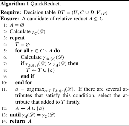
In the QuickReduct algorithm, Steps 5–10 are performed for improving the quality of classification. This algorithm uses a hill-climbing approach to obtain a candidate relative reduct by iteratively adding a condition attribute to the current candidate set. At each step, the attribute that maximizes the increase in the quality of approximation is selected. This hill-climbing strategy relies on the following property for determining the quality of classification.
Corollary 1. Let \(A\subseteq C\) be any subset of condition attributes, and \(a\in C\) be any condition attribute. The following inequality holds:
This corollary follows directly from Proposition 2, and its proof is omitted.
Example 2. The QuickReduct algorithm is applied to Table 1.
Omitting the detailed calculations, the following two relative reducts are obtained from Table 1 using the discernibility matrix and extraction method for all relative reducts: \(\{c_{1},c_{2},c_{3},c_{5}\}\) and \(\{c_{2},c_{3},c_{4},c_{5}\}\).
Notably, the QuickReduct algorithm may fail to produce a nonempty candidate relative reduct. For instance, in Example 1, the quality of classification using all condition attributes is \(\gamma_C(\mathscr{D})={5}/{14}\). However, for every single condition attribute \(c\in C\), the positive region \(Pos_{\{c\}}(\mathscr{D})\) is empty, and the corresponding quality of classification at Step 6 is \(\gamma_{\{c\}}(\mathscr{D})=0\).
In the case of condition attribute \(c_1\), the positive region \(Pos_{B}(\mathscr{D})\) and quality of classification \(\gamma_{B}(\mathscr{D})\) for the singleton \(B=\{c_{1}\}\) are as follows:
The same holds for the other condition attributes.
Therefore, if \(T=\emptyset\) and the termination condition at Step 13 is not satisfied, the QuickReduct algorithm cannot return the resulting set \(A\).
2.6. Variable Precision Rough Set
The VPRS model is a mathematical extension of Pawlak’s rough set theory 3. VPRS is based on a majority inclusion relation that uses the degree of misclassification, defined as follows.
Definition 9. Let \(X,Y\subseteq U\) be any sets of objects. The degree of misclassification \(c(X,Y)\) is defined as
Let \(\beta\in[0,0.5)\) be a parameter called the admissible classification error. The majority inclusion relation \(\stackrel{\beta}{\subseteq}\) is defined by
Clearly, the majority inclusion relation reduces to the standard set-theoretic inclusion when \(\beta=0\) 3.
The \(\beta\)-lower approximation \(\underline{A}_{\beta}(D_{i})\) of the decision class \(D_i\) is defined as follows.
Definition 10. Let \(DT=(U, C\cup D, V, \rho)\) be a decision table, \(A\subseteq C\) be any set of condition attributes, \(D_{i}\in\mathscr{D}\) be any decision class, and \(\beta\in[0,0.5)\) be the admissible classification error. The \(\beta\)-lower approximation \(\underline{A}_{\beta}(D_{i})\) of \(D_{i}\) with respect to \(A\) with \(\beta\) is defined as
Similar to the positive region and quality of classification in Pawlak’s rough set theory, the \(\beta\)-positive region \(Pos_{A}^{\beta}(\mathscr{D})\) and \(\beta\)-quality of classification \(\gamma_{A}^{\beta}(\mathscr{D})\) based on the admissible classification error \(\beta\) are respectively defined as follows.
Definition 11. Let \(A\subseteq C\) be a nonempty set of condition attributes, and \(\beta\in[0,0.5)\) be the admissible classification error. The \(\beta\)-positive region \(Pos_{A}^{\beta}(\mathscr{D})\) and \(\beta\)-quality of classification \(\gamma_{A}^{\beta}(\mathscr{D})\) are defined as
The \(\beta\)-positive region \(Pos_{A}^{\beta}(\mathscr{D})\) is the set of objects that can be classified into some decision class using the information in \(A\) in the admissible classification error \(\beta\in[0,0.5)\). Moreover, the \(\beta\)-quality of classification \(\gamma_{A}^{\beta}(\mathscr{D})\) is a measure of the correctness of the classification into decision classes based on \(\beta\in[0,0.5)\).
Note that, when \(\beta=0\), the notation is simplified to \(Pos_{A}(\mathscr{D})\) and \(\gamma_{A}(\mathscr{D})\) for the \(\beta\)-positive region and \(\beta\)-quality of classification. Note also that in Pawlak’s rough set theory, although the monotonicity of the positive regions and the quality of classification are generally guaranteed by Propositions 1 and 2, these properties may not be satisfied in VPRS. The following example illustrates this situation.
Example 3. Let the admissible classification error be \(\beta=0.3\) and \(A=\{c_{3}, c_{5}\}\). The equivalence classes by the indiscernibility relation \(R_{A}\) and \(\beta\)-positive region \(Pos_{A}^{\beta}(\mathscr{D})\) are constructed as follows:
-
・
\((c_{3}=0)\wedge(c_{5}=1)\rightarrow(d=1)\),
\(\hspace{1em}Cer(\cdot)={3}/{4},\;Cov(\cdot)={3}/{7},\;Supp(\cdot)={3}/{14},\)
-
・
\((c_{3}=0)\wedge(c_{5}=0)\rightarrow(d=2),\)
\(\hspace{1em}Cer(\cdot)=1,\;Cov(\cdot)={1}/{7},\;Supp(\cdot)={1}/{14}.\)
In this case, only one decision rule exists for each decision class. Although the decision rule for \(D_{2}\) is applicable to only one object in \(D_{2}\), in the case of the decision rule for \(D_{1}\), three of the seven objects in \(D_{1}\) satisfy this decision rule. This indicates that this rule represents part of the common relationship among the attribute values of \(c_{3}\), \(c_{5}\), and \(d\) for \(D_{1}\).
Suppose \(B=A\cup\{c_{4}\}=\{c_{3},c_{4},c_{5}\}\), then clearly, \(A\subseteq B\). However, given that the equivalence classes by \(R_{B}\) and \(\beta\)-positive region \(Pos_{B}^{\beta}(\mathscr{D})\) are constructed as follows:
Note that the following three decision rules are obtained from \(B\) with \(Cer(\cdot)\geq 1-\beta=0.7\):
-
・
\((c_{3}=0)\wedge(c_{4}=0)\wedge(c_{5}=1)\rightarrow(d=1),\)
\(\hspace{1em}Cer(\cdot)=1,\;Cov(\cdot)={1}/{7},\;Supp(\cdot)={1}/{14},\)
-
・
\((c_{3}=0)\wedge(c_{4}=1)\wedge(c_{5}=0)\rightarrow(d=2),\)
\(\hspace{1em}Cer(\cdot)=1,\;Cov(\cdot)={1}/{7},\;Supp(\cdot)={1}/{14},\)
-
・
\((c_{3}=1)\wedge(c_{4}=1)\wedge(c_{5}=1)\rightarrow(d=2),\)
\(\hspace{1em}Cer(\cdot)=1,\;Cov(\cdot)={1}/{7},\;Supp(\cdot)={1}/{14}.\)
As a result of using \(B\) by adding attribute \(c_{4}\) to \(A\), the antecedents of the decision rules can be used to describe more detailed conditions. However, in this case, it does not contribute to more accurate characterizations of between conditions and decisions. For \(D_{1}\), although the number of decision rules is the same, this decision rule explains only one object of \(D_{1}\); therefore, the common relationship describable by one decision rule using \(A\) is lost. This indicates that the description ability of \(D_{1}\) by decision rules decreases when \(c_{4}\) is added to \(A\).
Example 3 also illustrates that attributes such as \(c_{4}\) in \(B\) may lower the effectiveness of the decision rules obtained from a subset of condition attributes as a result of various types of attribute reduction. This indicates the importance and usefulness of redundancy checking and construction of true results in attribute reduction with no redundancy.
2.7. \(\beta\)-Reduct
Beynon 5 proposed the concept of \(\beta\)-reduct as a form of attribute reduction in VPRS.
Definition 12. A \(\beta\)-reduct is a nonempty set of condition attributes \(A\subseteq C\;(A\neq\emptyset)\) that satisfies the following two conditions based on the admissible classification error \(\beta\in[0,0.5)\):
-
1.
\(\gamma_{A}^{\beta}(\mathscr{D})=\gamma_{C}^{\beta}(\mathscr{D})\),
-
2.
\(\not\exists B\subset A,\;B\neq\emptyset\) and \(\gamma_{B}^{\beta}(\mathscr{D})=\gamma_{C}^{\beta}(\mathscr{D})\).
In this paper, \(\beta\)-reduct is defined as a nonempty minimal set \(A\subseteq C\) of condition attributes. This set preserves the \(\beta\)-quality of classification \(\gamma_{A}^{\beta}(\mathscr{D})\) compared with the \(\gamma_{C}^{\beta}(\mathscr{D})\) calculated using all condition attributes \(C\) based on the admissible classification error \(\beta\in[0,0.5)\). This definition prevents the empty set \(A\,(=\emptyset)\subset C\) from satisfying the \(\beta\)-reduct criteria. Note that in Beynon’s original definition of \(\beta\)-reduct, there are no explicit requirements for \(A\neq\emptyset\) and \(B\neq\emptyset\).
2.8. \(\hat{\beta}\)-Reduct
Nakahama et al. 18 proposed the concept of \(\hat{\beta}\)-reduct as an improvement to \(\beta\)-reduct.
Definition 13. A \(\hat{\beta}\)-reduct is a nonempty set of condition attributes \(A\subseteq C\;(A\neq\emptyset)\) satisfying the following two conditions based on the admissible classification error \(\beta\in[0,0.5)\):
-
1.
\(\gamma_{A}^{\beta}(\mathscr{D})\geq\gamma_{C}^{\beta}(\mathscr{D})\),
-
2.
\(\not\exists B\subset A,\;B\neq\emptyset\) and \(\gamma_{B}^{\beta}(\mathscr{D})\geq\gamma_{C}^{\beta}(\mathscr{D})\).
Based on the definitions of \(\beta\)-reduct and \(\hat{\beta}\)-reduct, it is clear that every \(\beta\)-reduct is also a \(\hat{\beta}\)-reduct. A \(\hat{\beta}\)-reduct is a set of condition attributes that not only preserves the \(\beta\)-quality of classification but also increases the value of the \(\beta\)-quality of classification compared with \(\gamma_{C}^{\beta}(\mathscr{D})\).
The following properties hold for \(\hat{\beta}\)-reduct 18.
Theorem 1. If \(\beta=0\), the definition of \(\hat{\beta}\)-reduct is identical to the definition of a relative reduct.
Theorem 2. If the decision table is consistent, the definition of \(\hat{\beta}\)-reduct is identical to the definition of a \(\beta\)-reduct.
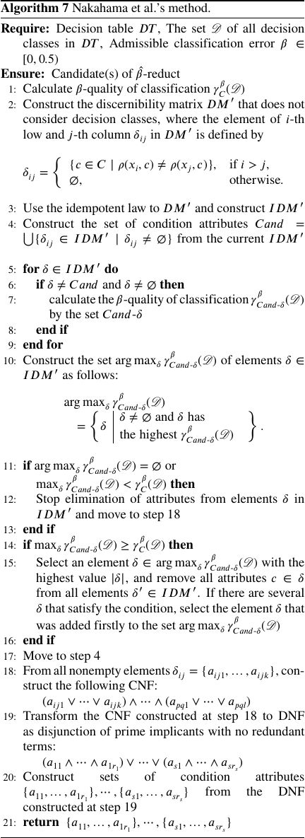
Nakahama et al. also proposed a heuristic algorithm for \(\hat{\beta}\)-reduct candidate calculation. The details of Nakahama et al.’s method are presented in Algorithm 7 in Appendix B. The algorithm was evaluated on eight datasets obtained from UCI ML Repository 22. All the candidates extracted by Nakahama et al.’s method from the decision tables using these datasets were confirmed to be \(\hat{\beta}\)-reducts 18. However, Nakahama et al.’s method relies on constructing and updating a discernibility matrix, generating a CNF from the discernibility matrix, and transforming the CNF into a DNF, which is a well-known NP-hard problem. Consequently, this method incurs a high computational cost.
3. A Refinement of the \(\hat{\beta}\)-QuickReduct Algorithm
In this section, a heuristic algorithm called \(\hat{\beta}\)-QuickReduct 19, which extracts a candidate \(\hat{\beta}\)-reduct by modifying the QuickReduct algorithm, is described. Then, a refined version of the \(\hat{\beta}\)-QuickReduct algorithm is proposed by introducing a confirmation process that verifies the original output of \(\hat{\beta}\)-QuickReduct and generates a valid \(\hat{\beta}\)-reduct from it if the original output does not constitute a candidate \(\hat{\beta}\)-reduct.
3.1. Details of the \(\hat{\beta}\)-QuickReduct Algorithm
The details of the \(\hat{\beta}\)-QuickReduct algorithm are presented in Algorithm 2. This algorithm is a slightly modified version of the original \(\hat{\beta}\)-QuickReduct algorithm proposed by Kudo and Okawa 19; however, the two algorithms are functionally identical.
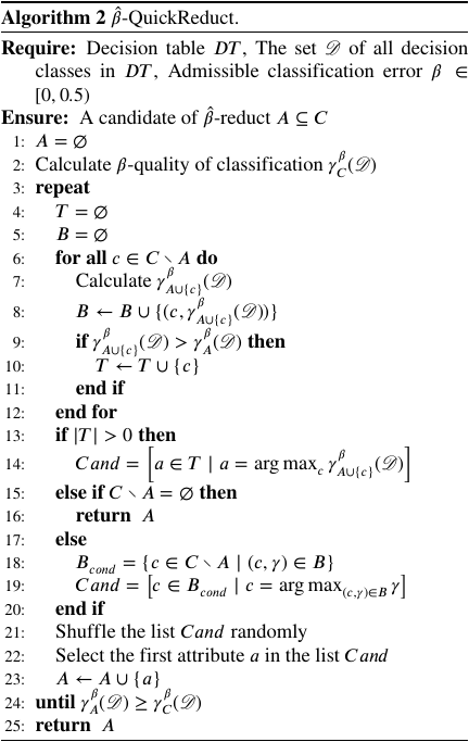
Note that Steps 14 and 19 construct the lists \(Cand\) of attributes \(c\in C\) that satisfy the required conditions, arranged in ascending order of attribute index. Note also that Step 21 is intended to increase the possibility that Algorithm 2 outputs different candidates of \(\hat{\beta}\)-reduct in each execution when multiple candidates exist.
Parts of Algorithm 2 are similar to those of the original QuickReduct algorithm. From Steps 6 to 12, for each condition attribute \(c\in C\setminus A\) that is not included in the current candidate \(\hat{\beta}\)-reduct \(A\), it is evaluated whether adding \(c\) to the current candidate \(A\) increases the current \(\beta\)-quality of classification \(\gamma_{A}^{\beta}(\mathscr{D})\). If adding \(c\) to \(A\) increases the value of \(\gamma_{A}^{\beta}(\mathscr{D})\), then \(c\) is added to the set \(T\) as a candidate attribute for inclusion in \(A\). If one or more candidate attributes for inclusion in \(A\) exist, then, in Step 22, one attribute \(a\) is selected from \(T\) and added to \(A\). These steps are repeated until \(A\) satisfies the termination condition in Step 24. Once \(A\) satisfies the termination condition, Algorithm 2 outputs \(A\) as a candidate \(\hat{\beta}\)-reduct.
The following distinctive features of the \(\hat{\beta}\)-QuickReduct algorithm are distinct from those of the original QuickReduct:
- 1.
- 2.
- 3.
Differences 1 and 3 are natural variations of the original QuickReduct algorithm because the purpose of Algorithm 2 is to obtain a candidate \(\hat{\beta}\)-reduct from the decision table \(DT\). Difference 2 is significant. In the VPRS model, the \(\beta\)-positive region and \(\beta\)-quality of classification do not generally satisfy the properties described in Propositions 1 and 2. Consequently, adding a condition attribute to the current candidate \(\hat{\beta}\)-reduct may decrease the \(\beta\)-quality of classification, which may lead to the following situation:
Therefore, the \(\hat{\beta}\)-QuickReduct algorithm must handle the case described in Eq. (20). Accordingly, in Step 8 of Algorithm 2, pairs \((c,\gamma_{A\cup\{c\}}^{\beta}(\mathscr{D}))\) are evaluated, for all condition attributes \(c\in C\setminus A\), where \(A\cup\{c\}\) is the set obtained by adding \(c\) to the current candidate \(A\). If there exists at least one candidate \(c\in T\), then, the list \(Cand\) of attributes to be added to the current set \(A\) is constructed in step 14 by selecting the attributes that increase the current value of \(\beta\)-quality of classification and yield the maximum value when added to \(A\). Otherwise, if no condition attribute increases the current \(\beta\)-quality of classification, then in Steps 18 and 19, the set \(B_{cond}\) of condition attributes is constructed from all pairs in \(B\). In addition, a list \(Cand\) of attributes to be added to the current set \(A\) is formed as the “second-best” attributes, which either preserve the current \(\beta\)-quality of classification or minimize its decrease.
The worst-case time computational complexity of Algorithm 2 was also analyzed. First, the number of processing steps in Step 2 was examined. Specifically, Step 2 consists of the following four processes: (1)sorting the entire dataset using counting sort based on each condition attribute \(c\in C\), (2)constructing the partition \(U/C\) from the sorted dataset, (3)constructing the \(\beta\)-lower approximations \(\underline{C}_{\beta}(D_{i})\;(D_{i}\in\mathscr{D})\), and (4)calculating the sum \({|\underline{C}_{\beta}(D_{i})|}/{|U|}\). Because counting sort is stable for discrete data, it can be solved in linear time with \(|U|\). However, the sorting of \(U\) requires computing the \(\beta\)-quality of classification \(\gamma_{C}^{\beta}(\mathscr{C})\) using every condition attribute \(c\in C\), which means that the computation process of (1) requires \(|U|\times|C|\) steps. Process (2) also requires \(|U||C|\) steps. Process (3) can be performed simultaneously with process (2). Finally, process (4) requires \(\sum_{D_i\mathscr{D}}|\underline{C}(D_{i})|\leq|U||C|\) steps at most. Thus, the total number of processing steps in Step 2 is at most \(3|U||C|\).
Next, the number of processing steps in the for loop (Steps 6–12) is examined. Because this loop calculates the \(\beta\)-quality of classification \(\gamma_{A\cup\{c\}}^\beta(\mathscr{D})\) for all \(c\in C\setminus A\), it requires at most \(|C|\times|U||C|=|U||C|^{2}\) steps. Steps 14 and 19 require a maximum of \(|U||C|^{2}\) steps each.
Moreover, in the worst-case scenario, achieving the termination condition \(\gamma_{A}^{\beta}(\mathscr{D}) \geq \gamma_{C}^{\beta}(\mathscr{D})\) in Step 24 requires the case \(A=C\), which means that Steps 3 to 24 be iterated \(|C|\) times, indicating that \(|C| \times |U||C|^{2}\) steps are required. All other steps have a constant time complexity \(O(1)\). Therefore, the overall time complexity of Algorithm 2 (\(\hat{\beta}\)-QuickReduct) is
Note that the output of the \(\hat{\beta}\)-QuickReduct algorithm is not guaranteed to be a true \(\hat{\beta}\)-reduct because no mechanism exists to ensure that Condition 2 in the definition of a \(\hat{\beta}\)-reduct is satisfied, even though Condition 1 is guaranteed by the termination condition in Step 24 in Algorithm 2. In Example 4, a case where the output of \(\hat{\beta}\)-QuickReduct is not a \(\hat{\beta}\)-reduct is illustrated, and the next two subsections introduce an improvement that ensures the output of our approach fully satisfies the definition of a \(\hat{\beta}\)-reduct.
Example 4. The computation process for extracting a candidate \(\hat{\beta}\)-reduct from the decision table (Table 1) using the \(\hat{\beta}\)-QuickReduct algorithm is illustrated. Here, the admissible classification error is \(\beta=0.3\).
In Step 2, the \(\beta\)-quality of classification \(\gamma_{C}^{\beta}(\mathscr{D})\) using the set of all condition attributes \(C\) is calculated. To calculate \(\gamma_{C}^{\beta}(\mathscr{D})\), the universe of discourse \(U=\{x_{1},\ldots,x_{14}\}\) is first sorted according to each condition attribute in \(C\) as follows:
From this sorting result, the following equivalence classes are obtained:
Example 1 illustrates the decision classes \(D_{1}\) and \(D_{2}\). The \(\beta\)-lower approximations of \(D_{1}\) and \(D_{2}\) with respect to \(C\) are
Therefore, the \(\beta\)-quality of classification \(\gamma_{C}^{\beta}(\mathscr{D})\) is \(\gamma_{C}^{\beta}(\mathscr{D}) = {3}/{14}+{2}/{14}={5}/{14}\).
The repeat-until loop starts with the current set \(A=\emptyset\). In this first iteration, \(\gamma_{\{c_{j}\}}^{\beta}(\mathscr{D})\) is calculated based on the equivalence classes \([x_{i}]_{\{c_{j}\}}\) \((i \in \{1,\ldots,14\}\), and \(j\in\{1,\ldots,5\}\)). However, \(\gamma_{\{c_{j}\}}^{\beta}(\mathscr{D})= 0\) for all condition attributes \(c_{j}\in C\), whereby \(Cand\) becomes the list of all condition attributes in Step 19. Here, we assume that attribute \(c_{1}\) is selected in Step 22 and candidate set \(A\) is updated to \(A=\{c_{1}\}\) in Step 23.
In the next loop, \(\gamma_{B_{j}}^{\beta}(\mathscr{D})\) is calculated for each set \(B_{j}=\{c_{1},c_{j}\}\) \(\;(j=2,3,4,5)\). The calculation results are as follows:
In the third loop, \(\gamma_{B_{j}}^{\beta}(\mathscr{D})\) is calculated for each set \(B_{j}=\{c_{1}, c_{2}, c_{j}\}\) \(\;(j=3,4,5)\). The calculation results are as follows:
In the fourth loop, \(\gamma_{B}^{\beta}(\mathscr{D})\) is calculated for the candidates formed by adding either \(c_{4}\) or \(c_{5}\) to \(A=\{c_{1},c_{2},c_{3}\}\) to determine the next attribute to be added to \(A\). The calculation results of the \(\beta\)-quality of classification for this selection are as follows:
Moreover, the updated \(A\) archives the \(\beta\)-quality of classification \(\gamma_{A}^{\beta}(\mathscr{D})=\gamma_{C}^{\beta}(\mathscr{D})={5}/{14}\). Therefore, the \(\hat{\beta}\)-QuickReduct algorithm outputs \(A=\{c_{1},c_{2},c_{3},c_{5}\}\) as a candidate \(\hat{\beta}\)-reduct.
Based on \(A=\{c_{1},c_{2},c_{3},c_{5}\}\), 11 decision rules were obtained from Table 1, and the averages of certainty, coverage, and support of these 11 decision rules were 0.727, 0.182, and 0.091, respectively. For eight of the 11 decision rules, there was just one object that satisfied the decision rule. Therefore, a decision rule does not describe the information about other objects in the same decision class. Thus, from the viewpoint of illustrating characteristics between conditions and decisions, the descriptive ability of these decision rules may not be useful. Examples of decision rules with \(Cer(\cdot)\geq 1-\beta=0.7\) are provided below:
-
・
\((c_{1}=0)\wedge(c_{2}=0)\wedge(c_{3}=0)\wedge(c_{5}=1)\rightarrow(d=1),\)
\(\hspace{1em}Cer(\cdot)=1,\;Cov(\cdot)={1}/{7},\;Supp(\cdot)={1}/{14},\)
-
・
\((c_{1}=0)\wedge(c_{2}=0)\wedge(c_{3}=1)\wedge(c_{5}=1)\rightarrow(d=1),\)
\(\hspace{1em}Cer(\cdot)=1,\;Cov(\cdot)={1}/{7},\;Supp(\cdot)={1}/{14},\)
-
・
\((c_{1}=1)\wedge(c_{2}=0)\wedge(c_{3}=0)\wedge(c_{5}=1)\rightarrow(d=1),\)
\(\hspace{1em}Cer(\cdot)=1,\;Cov(\cdot)={1}/{7},\;Supp(\cdot)={1}/{14},\)
-
・
\((c_{1}=0)\wedge(c_{2}=0)\wedge(c_{3}=0)\wedge(c_{5}=0)\rightarrow(d=2),\)
\(\hspace{1em}Cer(\cdot)=1,\;Cov(\cdot)={1}/{7},\;Supp(\cdot)={1}/{14},\)
-
・
\((c_{1}=1)\wedge(c_{2}=0)\wedge(c_{3}=1)\wedge(c_{5}=1)\rightarrow(d=2),\)
\(\hspace{1em}Cer(\cdot)=1,\;Cov(\cdot)={1}/{7},\;Supp(\cdot)={1}/{14}.\)
In Example 4, the output set \(A\) is not a \(\hat{\beta}\)-reduct because it does not satisfy the second condition of a \(\hat{\beta}\)-reduct, namely the minimality of set inclusion. Therefore, the \(\hat{\beta}\)-QuickReduct algorithm is refined by combining it with an additional procedure that verifies the output of \(\hat{\beta}\)-QuickReduct and generates a \(\hat{\beta}\)-reduct from its output if necessary.
3.2. Confirmation of the \(\hat{\beta}\)-Reduct
An algorithm, called CBHR (abbreviation for confirmation of \(\hat{\beta}\)-reduct) is proposed to verify whether the output of the \(\hat{\beta}\)-QuickReduct algorithm is indeed a \(\hat{\beta}\)-reduct of the given decision table. In practice, it can be difficult to determine whether a condition attribute \(c\in C\setminus A\) added to the current candidate set \(A\) of \(\hat{\beta}\)-reduct in Algorithm 2 will become a redundant attribute in the output of \(\hat{\beta}\)-QuickReduct. Therefore, an algorithm that examines the original output of \(\hat{\beta}\)-QuickReduct and produces a subset \(A'\subseteq A\) that is confirmed to be a \(\hat{\beta}\)-reduct is introduced.
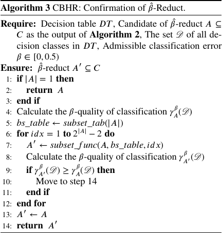
The details of the CBHR are presented in Algorithm 3. In this algorithm, nonempty proper subsets of the input candidate set \(A\) of a \(\hat{\beta}\)-reduct for the given \(DT\) are examined until either the smallest proper subset that fully satisfies the definition of a \(\hat{\beta}\)-reduct is found or \(A\) itself is confirmed as a \(\hat{\beta}\)-reduct.
In Algorithm 3, Steps 1–3 handle the case where \(A\) is a singleton because there is no need to remove redundant attributes in this case. Steps 5 and 7 constitute the core of this algorithm. These steps systematically select one of the smallest nonempty proper subsets \(A'\subset A\) to check whether \(A'\) qualifies as a \(\hat{\beta}\)-reduct. Selecting the smallest subset from all nonempty proper subsets is important in ensuring that the output of Algorithm 3 fully satisfies Condition 2 in the definition of a \(\hat{\beta}\)-reduct. As mentioned after Example 4, this selection is necessary because the output of \(\hat{\beta}\)-QuickReduct may not satisfy Condition 2, even though Condition 1 is guaranteed to be satisfied. Step 13 confirms that candidate \(A\) is a \(\hat{\beta}\)-reduct of the given decision table.
The algorithms subset_tab and subset_func are presented in Algorithms 4 and 5, respectively. Because the number of all nonempty proper subsets of a finite nonempty set \(A\) is \(2^{|A|}-2\), the algorithm assigns each nonempty proper subset of \(A\) a unique natural number \(i \in\{1,\ldots,2^{|A|}-2\}\). In Algorithm 4, Steps 2 and 3 represent each nonempty proper subset of \(A\) as an \(n\)-bit sequence, indicating whether each element \(e_{i}\;(1\leq i \leq n)\) of the given nonempty finite set \(F=\{e_{1},\ldots,e_{n}\}\) (the domain of \(A\)) belongs to the subset. Each nonempty proper subset is assigned a unique natural number to allow systematic handling. The \(i\)-th digit \(dig_{i}\) of the \(n\)-bit sequence is defined as
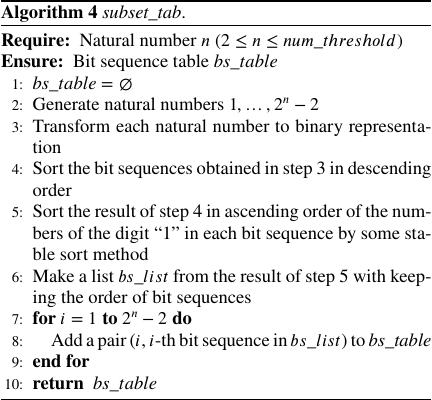
Steps 4 and 5 in Algorithm 4 are designed to reassign natural numbers to the subsets of \(A\) to control the assignment based on the size of the subsets and indices of their attributes. This reassignment ensures that subsets with smaller natural numbers correspond to smaller subset sizes and condition attribute indices.
The following proposition regarding subset_tab follows directly from its definition in Algorithm 4.
Proposition 3. Let bs_table be the output of the processes of subset_tab defined in Algorithm 4, and \(\mathbb{N}_{|{\it bs}\_{\it table}|}=\{n\in \mathbb{N}\;|\;1\leq n\leq |{\it bs}\_{\it table}|\}\) be the finite set of natural numbers. A one-to-one correspondence exists between the natural numbers in \(\mathbb{N}_{|{\it bs}\_{\it table}|}\) and the \(n\)-bit sequences that appear in bs_table.
The proof of Proposition 3 is omitted, as it is straightforward and follows from the construction process of subset_tab. The following proposition about subset_func supports our objective based on the definition of subset_tab in Algorithm 4.
Proposition 4. Let \(A\subseteq F\) be a finite nonempty subset of a finite domain \(F\) with \(|A|\geq 2\), and let subset_func be the procedure applied to \(A\) as defined in Algorithm 5. The following properties hold:
-
1.
subset_func is a surjection from the Cartesian product \((\mathscr{P}(F)\setminus\{\emptyset\})\times\) \({\it bs}\_{\it table}\times\mathbb{N}_{|{\it bs}\_{\it table}|}\) to the family \(\mathscr{P}(A)\setminus\{\emptyset, A\}\) of all nonempty proper subsets of \(A\), where \(\mathscr{P}(X)\) denotes the power set of a finite nonempty set \(X\).
-
2.
For any natural number \(i, j \in \mathbb{N}_{|{\it bs}\_{\it table}|}\), let \({\textit{subset}\_\textit{func}}(A, i)\) be denoted as \(A_{p}\), and \({\it subset}\_{\it func}(A, j)\) as \(A_{q}\). Then, \(|A_{p}| \leq |A_{q}|\) if and only if \(i\leq j\).
The proof of Proposition 4 is provided in Appendix A. The above discussion supports that the output of Algorithm 3 is a \(\hat{\beta}\)-reduct.
Theorem 3. Let \(DT\) be a decision table and let \(A\subseteq C\) be the output of Algorithm 2. Then, the output \(A'\subseteq A\) of Algorithm 3 is a \(\hat{\beta}\)-reduct of \(DT\).
The proof of Theorem 3 is provided in Appendix A.
Algorithm 3 considers the worst-case time computational complexity.
First, we examine the worst-case time complexity of Algorithm 4, which generates and sorts \(2^{n}-2\) numbers, resulting in a complexity of \(O(2^{n})\). In Algorithm 3, subset_tab is called with argument \(|A|\), and the for loop in Steps 6 to 12 is repeated \(2^{|A|}-2\) times in the worst case, to check for all nonempty proper subsets. Therefore, if the output of Algorithm 2 is \(C\), then the worst-case time complexity of Algorithm 3 is \(O(2^{|C|})\). However, in general, the number of attributes in the output set \(A\) of Algorithm 2 is much smaller than the total number of condition attributes. In Section 4, we show that this worst-case complexity does not considerably affect the average computation times in practice.
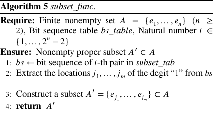
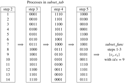
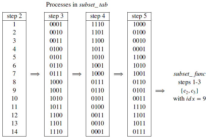
Fig. 1. Processes in subset_tab and subset_func for \(A=\{c_{1},c_{2},c_{3},c_{5}\}\) and \(idx=9\).
Example 5. As mentioned in Example 4, the output \(A=\{c_{1},c_{2},c_{3},c_{5}\}\) of \(\hat{\beta}\)-QuickReduct applied to Table 1 with an admissible classification error \(\beta=0.3\) is not a \(\hat{\beta}\)-reduct because it contains one or more redundant attributes. This example illustrates the process of confirming a \(\hat{\beta}\)-reduct from \(A\) using Algorithm 3.
In Algorithm 3, all nonempty proper subsets of the candidate set \(A\) are checked until either a subset of \(A\) is identified as a \(\hat{\beta}\)-reduct or \(A\) itself is confirmed as a \(\hat{\beta}\)-reduct by examining all nonempty proper subsets. Here, three cases with \(idx = 2,8,\) and \(9\) in the for loop of Algorithm 3 are described. The admissible classification error was set to \(\beta=0.3\).
Before entering the for loop (Steps 6–12), the \(\beta\)-quality of classification \(\gamma_{A}^{\beta}(\mathscr{D})\) is calculated for \(A=\{c_{1},c_{2},c_{3},c_{5}\}\), and the subset table bs_table is generated. In Step 4, \(\gamma_{A}^{\beta}(\mathscr{D})\) is calculated as follows.
Equivalence classes:
Because all equivalence classes are the same as in the final case of Example 4, the \(\beta\)-quality of classification for \(A\) is obtained as \(\gamma_{A}^{\beta}(\mathscr{D})={5}/{14}\).
Next, the subset table subset_tab with argument \(|A|=4\) is generated. The resulting subset table is shown in Fig. 1. In Algorithm 4, \(2^{|A|}-2=14\), and the natural numbers \(1,\ldots,14\) \(\in\mathbb{N}_{14}\) are generated in Step 2. Here, the parameter \(num\_\mathit{threshold}\) was assumed to be 16 in Algorithm 4.
In Step 3 of Algorithm 4, each natural number is converted into its binary representation, and the resulting list of binary representations is sorted in descending order in Step 4.
In Step 5, the sorted results are sorted again in ascending order using a stable sorting method, such as counting sort, based on the number of times the digit “1” appears in each binary representation. As a result of this step, the first four binary representations contain exactly one “1”; the next six representations contain two “1”s; and the last four representations contain three “1”s. Furthermore, the result preserves the order relationships among the first four representations from Step 4. The same applies to the next six and the last four representations.
The process returns to Algorithm 3, and the for loop in Steps 6–12 of Algorithm 3 is initiated. In the case of \(idx=2\), subset_func is called with the arguments \(A=\{c_{1},c_{2},c_{3},c_{5}\}\), the generated subset table \({\it bs}\_{\it table}\), and \(idx=2\) in Step 7. The second binary representation, “0100,” is selected based on \(idx=2\), and the set \(A'=\{c_{2}\}\) is constructed as a proper subset of the initial candidate \(A=\{c_{1},c_{2},c_{3},c_{5}\}\). The \(\beta\)-quality of classification for \(A'=\{c_{2}\}\) is then calculated in Step 8 of Algorithm 3. The equivalence classes are as follows:
The \(\beta\)-lower approximations are
\(\gamma_{A'}^{\beta}(\mathscr{D})\) is calculated as
Because the \(\beta\)-quality of classification \(\gamma_{A'}^{\beta}(\mathscr{D})=0\) when \(A'=\{c_{2}\}\) is less than \(\gamma_{A}^{\beta}(\mathscr{D})\), the termination condition in Step 9 is not satisfied, and the for loop continues.
Next, in Step 7, subset_func is called with the arguments \(A=\{c_{1},c_{2},c_{3},c_{5}\}\), \({\it bs}\_{\it table}\), and \(idx=8\) generating the proper subset \(A'=\{c_{2},c_{3}\}\) based on the eighth binary representation “0110.” The equivalence classes, \(\beta\)-lower approximations, and \(\beta\)-quality of classification based on \(A'=\{c_{2},c_{3}\}\) are as follows.
Equivalence classes:
The \(\beta\)-lower approximations and \(\beta\)-quality of classification:
Thus, the termination condition in Step 9 is still not satisfied for \(\{c_{2},c_{3}\}\), and the for loop is repeated.
Finally, the case where \(idx=9\) is described. In this case, a proper subset \(A'=\{c_{2},c_{5}\}\) based on the ninth binary representation “0101” is obtained. The equivalence classes, \(\beta\)-lower approximations, and \(\beta\)-quality of classification for \(A'=\{c_{2},c_{5}\}\) are as follows.
Equivalence classes:
The \(\beta\)-lower approximations and \(\beta\)-quality of classification:
Therefore, \(\gamma_{A'}^{\beta}(\mathscr{D})=\gamma_{A}^{\beta}(\mathscr{D})={5}/{14}\), and clearly, all nonempty proper subsets \(B \subset A'\) do not satisfy \(\gamma_{B}^{\beta}(\mathscr{D})=\gamma_{A}^{\beta}(\mathscr{D})\) because none of the cases with \(idx=1,\ldots,8\) satisfy the termination condition. This result confirms that \(A'=\{c_{2},c_{5}\}\) is a \(\hat{\beta}\)-reduct of Table 1.
From \(A'=\{c_{2},c_{5}\}\), seven decision rules were obtained. The averages of certainty, coverage, and support for these seven decision rules were 0.571, 0.286, and 0.143, respectively. The two decision rules with \(Cer(\cdot)\geq 1-\beta=0.7\) are described below:
-
・
\((c_{2}=0)\wedge(c_{5}=1)\rightarrow(d=1),\)
\(\hspace{1em}Cer(\cdot)={3}/{4},\;Cov(\cdot)={3}/{7},\;Supp(\cdot)={3}/{14},\)
-
・
\((c_{2}=0)\wedge(c_{5}=0)\rightarrow(d=2),\)
\(\hspace{1em}Cer(\cdot)=1,\;Cov(\cdot)={1}/{7},\;Supp(\cdot)={1}/{14}.\)
The decision rules thus obtained were compared with those in Example 4. The number of decision rules decreased from 11 to seven. Although the average certainty decreased, the average coverage and support increased when \(A=\{c_{1},c_{2},c_{3},c_{5}\}\) in Example 4. In decision rule for \(D_{1}\) with \(Cer(\cdot)\geq 0.7\), even though the antecedents of this rule “\((c_{2}=0)\wedge(c_{5}=1)\)” appear part of the antecedents of one decision rules for \(D_{2}\) in Example 4, this combination is common in all three rules for \(D_{1}\) with \(Cer(\cdot)\geq 0.7\) in Example 4. Therefore, the characteristics “\((c_{2}=0)\wedge(c_{5}=1)\)” illustrates the relationship of attribute values among \(c_{2}\), \(c_{5}\), and \(d\) appropriately.
For the decision class \(D_{2}\) with \(Cer(\cdot)\geq 0.7\), although the combination “\((c_{2}=0)\wedge(c_{5}=1)\)” disappears as an exception of the characteristics for \(D_{1}\) and the antecedents “\((c_{2}=0)\wedge(c_{5}=0)\)” appear only in an object in \(D_{2}\), the combination “\((c_{2}=0)\wedge(c_{5}=0)\)” describes an important characteristic for correctly classifiable object in \(D_{2}\).
3.3. Refined \(\hat{\beta}\)-QuickReduct Algorithm
An improvement of the \(\hat{\beta}\)-QuickReduct algorithm called “Refined \(\hat{\beta}\)-QuickReduct” is introduced by combining the original \(\hat{\beta}\)-QuickReduct algorithm with the CBHR algorithm. The Refined \(\hat{\beta}\)-QuickReduct is described in Algorithm 6.
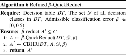
As shown in Algorithm 6, the working process of Refined \(\hat{\beta}\)-QuickReduct is straightforward. First, a candidate set \(A\) of a \(\hat{\beta}\)-reduct is generated by the original \(\hat{\beta}\)-QuickReduct. Next, \(A\) is verified and refined using the CBHR algorithm to produce \(A'\). Finally, \(A'\) is output as a \(\hat{\beta}\)-reduct.
The Refined \(\hat{\beta}\)-QuickReduct can reliably output a \(\hat{\beta}\)-reduct, as proposed by Theorem 3. As discussed in Sections 3.1 and 3.2 and in the proof of Theorem 3 in Appendix A, this is because the original \(\hat{\beta}\)-QuickReduct ensures that the output set \(A\) satisfies Condition 1 of the definition of a \(\hat{\beta}\)-reduct, and the CBHR algorithm ensures that the output \(A'\) satisfies Condition 2 of the same definition.
The worst-case time computational complexity of the Refined \(\hat{\beta}\)-QuickReduct algorithm can easily be confirmed to be of order \(O(2^{|C|})\) because the original \(\hat{\beta}\)-QuickReduct has complexity \(O(|U||C|^{3})\) and the CBHR algorithm has complexity \(O(2^{|C|})\). This means that the complexity of the CBHR algorithm dominates the overall worst-case complexity of the Refined \(\hat{\beta}\)-QuickReduct. However, as mentioned in Section 3.2, the impact of this worst-case complexity on average computation times is not significant, as demonstrated in Section 4.
4. Experiments
This section presents the following two experiments that we conducted.
Experiment 1: The original \(\hat{\beta}\)-QuickReduct (Algorithm 2), Refined \(\hat{\beta}\)-QuickReduct (Algorithm 6), and Nakahama et al.’s method (Algorithm 7 in Appendix B) are compared from the following viewpoints: success ratio of extracting \(\hat{\beta}\)-reduct(s), average number of attributes in the output, average score of the \(\beta\)-quality of classification of outputs, and average calculation time.
Experiment 2: Thirty outputs of the original \(\hat{\beta}\)-QuickReduct and Refined \(\hat{\beta}\)-QuickReduct were recalculated. From these results, decision rules were obtained, and the average values of the number of obtained decision rules, average length of antecedences (the number of condition attributes appearing in antecedences), certainty, coverage, and support were evaluated.
In both experiments, all the algorithms were applied to the eight datasets listed in Table 2. In Table 2, the attribute #objs, #conds, #dcs, and cst represent the number of objects, number of condition attributes, number of decision classes, and whether the decision table constructed from the dataset is consistent, respectively. Following the experiments of Nakahama et al. 18, the admissible classification error was set to \(\beta=0.3\). All experiments were performed on a Windows PC with OS Windows 11 Pro, CPU 11th Gen Intel® Core i5-1155G7 at 2.50 GHz, RAM 16 GB, and all experimental programs were implemented in Python 3.12.4.
Experiment 1: For each dataset, all methods were applied 30 times. In each run, the following points were checked and measured: whether a \(\hat{\beta}\)-reduct was extracted, the \(\beta\)-quality of classification, the number of attributes in the extracted results, and computation time. Because the measured values may be widely distributed, the original \(\hat{\beta}\)-QuickReduct and Refined \(\hat{\beta}\)-QuickReduct were each applied 30 times, and the average of 30 iterations was calculated. Note that this iteration is not required in Nakahama et al.’s method because no randomness is used in Nakahama et al.’s method, as in Algorithm 7, and therefore, Nakahama et al.’s method outputs the same result from the dataset.
| Dataset | #objs | #conds | #dcs | cst |
| Zoo | 101 | 16 | 7 | yes |
|
Breast Cancer (BC) |
287 | 9 | 2 | no |
| vote | 435 | 16 | 2 | yes |
|
Las Vegas Strip (LVS) |
504 | 19 | 5 | yes |
| Glioma (Gl) | 839 | 23 | 2 | no |
|
Tic-Tac-Toe (TTT) |
958 | 9 | 2 | yes |
|
Travel Reviews (TR) |
980 | 10 | 3 | no |
| car | 1728 | 6 | 4 | yes |
Tables 3 and 4 encapsulate the experimental results of the proposed method and Nakahama et al.’s method, respectively. In Table 3, the terms “\(\hat{\beta}\)-QR” and “R. \(\hat{\beta}\)-QR” are abbreviations for \(\hat{\beta}\)-QuickReduct and Refined \(\hat{\beta}\)-QuickReduct, respectively. In this table, except for the columns “CBHR,” the terms “\(\gamma_C^{\beta}\),” “suc. rat.,” “avg. attrs,” “avg. gam.,” and “total avg. t.” refer to the \(\beta\)-quality of classification of the decision table constructed from each dataset by \(C\) with \(\beta=0.3\), the success ratio of extracting \(\hat{\beta}\)-reduct (unit: \(\%\)), average number of attributes in the candidates (or \(\hat{\beta}\)-reducts) extracted by the algorithms, average value of \(\beta\)-quality of classification for the extracted candidates (or \(\hat{\beta}\)-reducts), and average total computation time of Refined \(\hat{\beta}\)-QuickReduct (unit: second), respectively. In the columns “CBHR,” the term “avg. t.” and “rat.” refer to the average computation time (unit: second) of the CBHR algorithm in the total computation time of Refined \(\hat{\beta}\)-QuickReduct, and the ratio of the average computation time (unit: \(\%\)) of CBHR algorithm in the average total computation time of Refined \(\hat{\beta}\)-QuickReduct, respectively. The symbol “*” indicates significant differences between the average computation times of the Refined \(\hat{\beta}\)-QuickReduct and Nakahama et al.’s method with a probability \(p<0.01\). Similarly, in Table 4, the terms “#cand.,” “suc. ratio [\(\%\)],” “avg. time [s],” “attrs,” and “avg. gamma” refer to the number of candidate \(\hat{\beta}\)-reducts, the success ratio of extracting \(\hat{\beta}\)-reduct(s) (unit: \(\%\)), average computation time of Nakahama et al.’s method (unit: second), average number of attributes in the extracted \(\hat{\beta}\)-reduct(s) by the algorithms, and average value of \(\beta\)-quality of classification for the extracted \(\hat{\beta}\)-reduct(s), respectively.
Experiment 2: After Experiment 1, 30 outputs were obtained again for each dataset using the original \(\hat{\beta}\)-QuickReduct and Refined \(\hat{\beta}\)-QuickReduct. In Experiment 2, the decision rules are constructed from the outputs, and the obtained decision rules are evaluated by the five criteria mentioned above.
Table 5 presents the extraction results of the decision rules from the output of \(\hat{\beta}\)-QuickReduct and Refined \(\hat{\beta}\)-QuickReduct. In Table 5, similar to the case of Table 3, the terms “\(\hat{\beta}\)-QR” and “R. \(\hat{\beta}\)-QR” are abbreviations for \(\hat{\beta}\)-QuickReduct and Refined \(\hat{\beta}\)-QuickReduct, respectively. The terms “avg. #dec. r.,” “avg. r. len.,” “avg. cer.,” “avg. cov.,” and “avg. supp.” refers to the average number of extracted decision rules, average length (number of condition attributes appeared in antecedents) of extracted decision rules, average scores of certainty, coverage, and support of the extracted decision rules, respectively.
| Dataset | \(\gamma_{C}^{\beta}\) | \(\hat{\beta}\)-QR | R. \(\hat{\beta}\)-QR | |||||||
| suc. | avg. | avg. | suc. | total | CBHR | avg. | avg. | |||
| rat. | attrs | gam. | rat. | avg. t. | avg. t. | rat. | attrs | gam. | ||
| zoo | 1.0 | 73.33 | 3.67 | 1.0 | 100 | \(0.014^{*}{\pm}0.008\) | 0.003 | 0.190 | 3.4 | 1.0 |
| BC | 0.955 | 0 | 9 | 0.955 | 100 | \(0.666^{*}{\pm}0.017\) | 0.624 | 0.936 | 8 | 0.995 |
| vote | 1.0 | 100 | 1 | 1.0 | 100 | \(0.010^{*}{\pm}0.008\) | \(9.64\mathrm{e}^{-5}\) | 0.009 | 1 | 1.0 |
| LSV | 1.0 | 100 | 3 | 1.0 | 100 | \(0.148^{*}{\pm}0.010\) | 0.017 | 0.117 | 3 | 1.0 |
| Gl | 0.920 | 100 | 1 | 1.0 | 100 | \(0.029^{*}{\pm}0.006\) | \(4.05\mathrm{e}^{-4}\) | 0.014 | 1 | 1.0 |
| TTT | 1.0 | 100 | 8 | 1.0 | 100 | \(0.871^{*}{\pm}0.023\) | 0.722 | 0.829 | 8 | 1.0 |
| TR | 0.894 | 100 | 1 | 1.0 | 100 | \(0.019^{*}{\pm}0.004\) | \(4.2\mathrm{e}^{-5}\) | 0.002 | 1 | 1.0 |
| car | 1.0 | 100 | 6 | 1.0 | 100 | \(1.257^{*}{\pm}0.011\) | 0.798 | 0.637 | 6 | 1.0 |
| \(^{*}:p<0.01\) | ||||||||||
| Dataset | #cand. | suc. ratio [%] | avg. time [s] | attrs | avg. gamma |
| zoo | 1 | 100 | \(0.354{\pm}0.020\) | 3 | 1.0 |
| BC | 1 | 100 | \(1.435{\pm}0.026\) | 8 | 0.955 |
| vote | 1 | 100 | \(78.324{\pm}1.390\) | 1 | 1.0 |
| LSV | 1 | 100 | \(59.464{\pm}1.031\) | 6 | 1.0 |
| Gl | 1 | 100 | \(273.140{\pm}26.399\) | 1 | 1.0 |
| TTT | 8 | 100 | \(8.571{\pm}0.185\) | 8 | 1.0 |
| TR | 1 | 100 | \(2.343{\pm}0.084\) | 1 | 1.0 |
| car | 1 | 100 | \(4.866{\pm}0.096\) | 6 | 1.0 |
| Dataset | \(\hat{\beta}\)-QR | R. \(\hat{\beta}\)-QR | ||||||||
| avg. | avg. | avg. | avg. | avg. | avg. | avg. | avg. | avg. | avg. | |
| #dec. r. | r. len. | cer. | cov. | supp. | #dec. r. | r. len. | cer. | cov. | supp. | |
| zoo | 19.4 | 3.67 | 0.611 | 0.376 | 0.054 | 18.6 | 3.4 | 0.767 | 0.397 | \(0.057\) |
| BC | 272 | 9 | 0.978 | 0.007 | 0.004 | 268 | 8 | 0.978 | 0.007 | 0.007 |
| vote | 6 | 1 | 0.5 | 0.333 | 0.167 | 6 | 1 | 0.5 | 0.333 | 0.167 |
| LSV | 503 | 1 | 1 | 0.010 | 0.002 | 503 | 3 | 1 | 0.010 | 0.002 |
| Gl | 4 | 1 | 0.5 | 0.5 | 0.250 | 4 | 1 | 0.5 | 0.5 | 0.250 |
| TTT | 958 | 8 | 1 | 0.002 | 0.001 | 958 | 8 | 1 | 0.002 | 0.001 |
| TR | 6.9 | 1 | 0.393 | 0.549 | 0.183 | 6.9 | 1 | 0.393 | 0.549 | 0.183 |
| car | 1728 | 6 | 1 | 0.002 | 0.001 | 1728 | 6 | 1 | 0.002 | 0.001 |
5. Discussion
First, the results of Experiment 1 are discussed. As mentioned in Section 3.3, Refined \(\hat{\beta}\)-QuickReduct can reliably extract a \(\hat{\beta}\)-reduct. This property is theoretically supported and confirmed by the experimental results in Table 3, which show that the success ratio of the extractions by Refined \(\hat{\beta}\)-QuickReduct was \(100\%\) for every dataset. The average computation times of Refined \(\hat{\beta}\)-QuickReduct were significantly faster than those of Nakahama et al.’s method across all datasets.
The results of “rat.” in CBHR columns and “avg. attrs” show a clear tendency that the larger the number of attributes in the extracted \(\hat{\beta}\)-reduct is, the larger the ratio of the computation time of the CBHR algorithm is in the Refined \(\hat{\beta}\)-QuickReduct algorithm (Pearson’s correlation coefficient \(r=0.986\)). This fact indicates that if the output of \(\hat{\beta}\)-QuickReduct, \(\hat{\beta}\)-reduct candidate is small, in particular, if the candidate is a singleton, the computation time of the CBHR algorithm is very short, and the ratio of this computation time to the total computation time is very small. In the case that the \(\hat{\beta}\)-reduct candidate is not small, the computation time of the CBHR algorithm increases, and the ratio of the CBHR algorithm computation time to the total computation time of the Refined \(\hat{\beta}\)-QuickReduct also increases. This is because the CBHR algorithm systematically calculates a nonempty proper subset of the \(\hat{\beta}\)-reduct candidate until it finds a nonempty proper subset as a true \(\hat{\beta}\)-reduct or confirms the \(\hat{\beta}\)-reduct candidate to be a true \(\hat{\beta}\)-reduct by checking all nonempty proper subsets. However, as mentioned above, even though the ratio of CBHR algorithm computation time is large, the total computation time of the Refined \(\hat{\beta}\)-QuickReduct is significantly shorter than that of Nakahama et al.’s method.
Moreover, for the Glioma and Travel Reviews datasets, the \(\hat{\beta}\)-reducts extracted by both the Refined \(\hat{\beta}\)-QuickReduct and Nakahama et al.’s method provided higher \(\beta\)-quality of classification values than the original values based on all condition attributes. These three observations demonstrate the effectiveness of the proposed approach for extracting \(\hat{\beta}\)-reducts.
However, as shown in Example 4, the original \(\hat{\beta}\)-QuickReduct may fail to extract a \(\hat{\beta}\)-reduct. In the experiments, in certain cases, the candidates extracted by the original \(\hat{\beta}\)-QuickReduct were not \(\hat{\beta}\)-reducts, specifically: eight out of 30 executions on the zoo-type dataset and all 30 executions on the Breast Cancer dataset. This tendency is consistent with the experimental results reported in 19. The main reason for these cases is that the attributes added to the candidate in the early steps later become redundant. Note that the number of attributes in the output of the original \(\hat{\beta}\)-QuickReduct corresponds to the number of loop repetitions between Steps 3 and 24 in Algorithm 2. For example, output \(A=\{c_{1},c_{2},c_{3},c_{5}\}\) in Example 4 contains four attributes that correspond to four iterations of the loop. In Example 5, the attributes \(c_{1}\) and \(c_{3}\) were removed by the CBHR algorithm, despite being added to the candidate \(\hat{\beta}\)-reduct in the first and third iterations.
In the zoo-type dataset in Experiment 1, all eight cases that failed to extract \(\hat{\beta}\)-reducts produced the same candidate \(A=\{c_{9}\) (backbone), \(c_{10}\) (breathes), \(c_{12}\) (fins), \(c_{13}\) (legs)\(\}\). However, the actual \(\hat{\beta}\)-reduct obtained by the CBHR algorithm was \(A'=\{c_{9}, c_{12}, c_{13}\}\). The attribute \(c_{10}\) was added to the candidate during the second loop of the four loops as the best attribute providing the highest \(\beta\)-quality of classification at that time, but it later became redundant because \(\gamma_{A'}^{\beta}(\mathscr{D})=\gamma_{A}^{\beta}(\mathscr{D})\).
Similarly, in all 30 failed cases of the Breast Cancer dataset, the output of the original \(\hat{\beta}\)-QuickReduct contained nine attributes, whereas the actual \(\hat{\beta}\)-reduct obtained by Refined \(\hat{\beta}\)-QuickReduct had eight attributes. The rejected attribute was added to the current candidate during the fourth loop of the nine repetitions. These observations highlight the necessity and rationality of applying the CBHR algorithm to the output of the original \(\hat{\beta}\)-QuickReduct and demonstrate the difficulty of predicting whether a selected attribute added to the current candidate may later become redundant, as discussed in Section 3.2.
Moreover, for any consistent decision table, Refined \(\hat{\beta}\)-QuickReduct outputs a \(\hat{\beta}\)-reduct with a \(\beta\)-quality of classification equal to \(1.0\) because \(\gamma_{C}^{\beta}(\mathscr{D})=1.0\) for any admissible classification error \(\beta\in [0,0.5)\) according to the termination condition in Step 24 of Algorithm 2, and the output \(A'\) of the CBHR algorithm satisfies \(\gamma_{A'}^{\beta}(\mathscr{D})\geq\gamma_{C}^{\beta}(\mathscr{D})\). From the perspective of discrete data analysis, in certain cases, a \(\hat{\beta}\)-reduct-like set of condition attributes with a slightly lower \(\beta\)-quality of classification than 1.0 is preferred. This represents an important application in real-data analysis for the practical consideration of the proposed approach.
Next, the results of Experiment 2 are discussed. Except for the zoo and BC datasets, all results of the six datasets in Table 5 are identical. This is because the extracted \(\hat{\beta}\)-reducts are identical between the original \(\hat{\beta}\)-QuickReduct and Refined \(\hat{\beta}\)-QuickReduct. Therefore, the decision rules obtained are also identical for these two methods.
On the BC dataset, in Tables 2 and 5, the number of objects is 287, and the number of decision rules is 272 for the original \(\hat{\beta}\)-QuickReduct and 268 for the Refined \(\hat{\beta}\)-QuickReduct. The result of the original \(\hat{\beta}\)-QuickReduct contains all nine condition attributes, which means that the original \(\hat{\beta}\)-QuickReduct could not remove the redundant condition attribute at all. However, the Refined \(\hat{\beta}\)-QuickReduct removed one condition attribute (inv-nodes), and the removed attribute had the most attribute values, that is, 13, which simplifies the meaning of the decision rules.
On the zoo dataset, the original \(\hat{\beta}\)-QuickReduct failed 11 of 30 cases to generate a true \(\hat{\beta}\)-reduct, and all 11 failed cases generated \(A=\{c_{9},\) \(c_{10},\) \(c_{12},\) \(c_{13}\}\), that is, \(c_{10}\) (breathes) was redundant. Set \(A\) generated 18 decision rules and the average values of certainty, coverage, and support were 0.833, 0.389, and 0.056, respectively. On the other hand, the Refined \(\hat{\beta}\)-QuickReduct extracted a true \(\hat{\beta}\)-reduct \(A'=\{c_{9}, c_{12}, c_{13}\}\) in 18 cases of the 30 repetitions of experiments. The result \(A'\) generated 15 decision rules. The average scores for certainty, coverage, and support of these 15 decision rules were 0.667, 0.467, and 0.067, respectively.
In 30 repetitions of the zoo experiment dataset, two types of true \(\hat{\beta}\)-reducts were extracted. Another true \(\hat{\beta}\)-reduct \(\{c_{4}, c_{6},\) \(c_{13}, c_{14}\}\) (meanings of attributes \(c_{4}\), \(c_{6}\), and \(c_{14}\) are omitted) was extracted 12 times by the Refined \(\hat{\beta}\)-QuickReduct, and this result generated 24 decision rules. The average scores for the certainty, coverage, and support of these 24 decision rules were 0.917, 0.292, and 0.042, respectively.
Moreover, although the difference of average numbers of condition attributes between the results of the original \(\hat{\beta}\)-reducts and the results of the Refined \(\hat{\beta}\)-reducts is not large, all the antecedents of the decision rules obtained from the results of the Refined \(\hat{\beta}\)-reducts did not contain the redundant condition attributes \(c_{10}\) in Experiment 2.
6. Conclusion
In this paper, an improved approach for \(\hat{\beta}\)-QuickReduct was proposed. The purpose of this improvement is to guarantee the extraction of a \(\hat{\beta}\)-reduct from a given decision table. The proposed algorithm, called Refined \(\hat{\beta}\)-QuickReduct, combines the original \(\hat{\beta}\)-QuickReduct algorithm with the CBHR algorithm to verify whether the output of the original \(\hat{\beta}\)-QuickReduct is a \(\hat{\beta}\)-reduct and to generate a \(\hat{\beta}\)-reduct if necessary. Refined \(\hat{\beta}\)-QuickReduct provides the following three advantages:
-
1.
The extraction of a \(\hat{\beta}\)-reduct is theoretically supported.
-
2.
Computation of \(\hat{\beta}\)-reduct is highly efficient.
-
3.
The \(\beta\)-quality of classification may be higher than the original value obtained using the full set of condition attributes.
The results of the comparison experiments with Nakahama et al.’s method confirm these advantages, and indicate the usefulness of reliably extracting a \(\hat{\beta}\)-reduct from the perspective of discrete table-style data analysis.
Future directions for the proposed approach include
-
1.
Automatic determination of an appropriate parameter value \(\beta\in[0,0.5)\) for a given decision table.
-
2.
Extraction of \(\hat{\beta}\)-reducts that achieve a slightly lower \(\beta\)-quality of classification than that obtained using the full set of condition attributes from consistent decision tables.
-
3.
Application of the proposed approach to real-world large-scale datasets.
Acknowledgments
The authors appreciate the anonymous AE and two reviewers for their helpful comments and suggestions. The authors also thank Mr. Yoshiki Nakahama who provided all the resources for Nakahama et al.’s method.
- [1] Z. Pawlak, “Rough sets,” Int. J. of Information and Computer Science, Vol.11, No.5, pp. 341-356, 1982. https://doi.org/10.1007/BF01001956
- [2] Z. Pawlak, “Rough Sets: Theoretical Aspects of Reasoning about Data,” Kluwer Academic Publishers, 1991. https://doi.org/10.1007/978-94-011-3534-4
- [3] W. Ziarko, “Variable precision rough set model,” J. of Computer and System Sciences, Vol.46, No.1, pp. 39-59, 1993. https://doi.org/10.1016/0022-0000(93)90048-2
- [4] J. D. Katzberg and W. Ziarko, “Variable Precision Extension of Rough Sets,” Fundamenta Informaticae, Vol.27, Nos.2-3, pp. 155-168, 1996. https://doi.org/10.3233/FI-1996-272304
- [5] M. Beynon, “Reducts within the variable precision rough sets model: A further investigation,” European J. of Operational Research, Vol.134, No.3, pp. 592-605, 2001. https://doi.org/10.1016/S0377-2217(00)00280-0
- [6] M. J. Beynon and M. J. Peel, “Variable precision rough set theory and data discretization: An application to corporate failure prediction,” Omega, Vol.29, No.6, pp. 561-576, 2001. https://doi.org/10.1016/S0305-0483(01)00045-7
- [7] C. T. Su and J. H. Hsu, “Precision parameter in the variable precision rough sets model: An application,” Omega, Vol.34, No.2, pp. 149-157, 2006. https://doi.org/10.1016/j.omega.2004.08.005
- [8] M. Inuiguchi, “Structure-Based Attribute Reduction in Variable Precision Rough Set Models,” J. Adv. Comput. Intell. Intell. Inform., Vol.10, No.5, pp. 657-665, 2006. https://doi.org/10.20965/jaciii.2006.p0657
- [9] X. Zhao, M. Ha, and A. Zhang, “Variable Precision Rough Set Model in Incomplete Ordered Decision System,” Proc. of 2008 3rd Int. Conf. Innovative Computing, Information and Control (ICICIC), Article No.498, 2008. https://doi.org/10.1109/ICICIC.2008.672
- [10] Y. Kudo and T. Murai, “A Heuristic Algorithm for Generating Decision Rules in Variable Precision Rough Set Models,” Proc. of SCIS & ISIS 2010, pp. 1568-1573, 2010. https://doi.org/10.14864/softscis.2010.0.1568.0
- [11] X. D. Song, J. W. Mu, R. F. Feng, and Z. Z. Qiu, “Variable Precision Rough Set Optimization Algorithm for Constructing Decision Tree,” Advanced Materials Research, Vols.181-182, pp. 43-48, 2011. https://doi.org/10.4028/www.scientific.net/AMR.181-182.43
- [12] Y. Weiguo, L. Mingyu, and L. Zhi, “Variable precision rough set based decision tree classifier,” J. of Intelligent & Fuzzy Systems, Vol.23, Nos.2-3, pp. 61-70, 2012. https://doi.org/10.3233/IFS-2012-0496
- [13] Y. Liu, Y. Lin, and H.-h. Zhao, “Variable precision intuitionistic fuzzy rough set model and applications based on conflict distance,” Expert Systems, Vol.32, No.2, pp. 220-227, 2015. https://doi.org/10.1111/exsy.12083
- [14] F. M. Perez, J. V. B. Martienz, A. F. Oliva, and M. A. Ortega, “Application of the Variable Precision Rough Sets Model to Estimate the Outlier Probability of Each Element,” Complexity, Vol.2018, No.1, Article No.4867607, 2018. https://doi.org/10.1155/2018/4867607
- [15] A. Apriani, I. T. R. Yanto, S. Fathurrohmah, S. Haryatmi, and D. Danardono, “Variable precision rough set model for attribute selection on environment impact dataset,” Int. J. of Advances in Intelligent Informatics, Vol.4, No.1, pp. 70-75, 2018. https://doi.org/10.26555/ijain.v4i1.109
- [16] B. Yu, Y. Hu, and J. Dai, “A bi-variable precision rough set model and its application to attribute reduction,” Information Sciences, Vol. 645, Article No.119368, 2023. https://doi.org/10.1016/j.ins.2023.119368
- [17] Z. T. Gong, B. Z. Sun, Y. B. Shao, D. G. Chen, and Q. He, “Variable precision rough set model based on general relation,” Proc. of 2024 Int. Conf. Machine Learning and Cybernetics, Vol.4, pp. 2490-2494, 2024. https://doi.org/10.1109/ICMLC.2004.1382222
- [18] Y. Nakahama, H. Okawa, Y. Kudo, and T. Murai, “An Improvement of β-reduct and Its Computation in Variable Precision Rough Set Model,” J. of the Japan Society for Fuzzy Theory and Intelligent Informatics, Vol.37, No.1, pp. 596-606, 2025 (in Japanese). https://doi.org/10.3156/jsoft.37.1_596
- [19] Y. Kudo and H. Okawa, “β̂-QuickReduct: A Heuristic Algorithm for Computing a β̂-Reduct Candidate in Variable Precision Rough Set Model,” Proc. of 41th Fuzzy System Symp. (FSS2025), 2025 (in Japanese). https://doi.org/10.14864/fss.41.0_563
- [20] A. Chouchoulas and Q. Shen, “Rough Set-Aided Keyword Reduction for Text Categorization,” Applied Artificial Intelligence, Vol.15, No.9, pp. 843-873, 2001. https://doi.org/10.1080/088395101753210773
- [21] A. Skowron and C. Rauser, “The discernibility matrix and functions in information systems,” R. Słowiński (Ed.), “Intelligent Decision Support. Theory and Decision Library,” pp. 331-362, Springer, 1992. https://doi.org/10.1007/978-94-015-7975-9_21
- [22] UCI Machine Learning Repository. http://archive.ics.uci.edu/ [Accessed October 1, 2019]
Appendix
Appendix A. Proofs of Theoretical Results
Proposition 4. Let \(A\subseteq F\) be a finite nonempty subset of a finite domain \(F\) with \(|A|\geq 2\), and let subset_func be the procedure applied to \(A\) as defined in Algorithm 5. The following properties hold:
-
1.
subset_func is a surjection from the Cartesian product \((\mathscr{P}(F)\setminus\{\emptyset\})\times\) \({\it bs}\_{\it table}\times\mathbb{N}_{|{\it bs}\_{\it table}|}\) to the family \(\mathscr{P}(A)\setminus\{\emptyset, A\}\) of all nonempty proper subsets of \(A\), where \(\mathscr{P}(X)\) denotes the power set of a finite nonempty set \(X\).
-
2.
For any natural number \(i, j \in \mathbb{N}_{|{\it bs}\_{\it table}|}\), let \({\it subset}\_{\it func}(A, i)\) denote \(A_{p}\), and \({\it subset}\_{\it func}(A, j)\) denote \(A_{q}\). Then, \(|A_{p}| \leq |A_{q}|\) if and only if \(i\leq j\).
Proof. Proof of Property 1:
First, we prove that subset_func is a function that maps \((\mathscr{P}(F)\setminus\{\emptyset\})\times\) \({\it bs}\_{\it table}\times\mathbb{N}_{|{\it bs}\_{\it table}|}\) to \(\mathscr{P}(A)\setminus\{\emptyset, A\}\), and for every nonempty proper subset \(A' \subset A\), there exists a triple \((A, (i,bs_{i}), i) \in (\mathscr{P}(F)\setminus\{\emptyset\})\times\) \({\it bs}\_{\it table}\times\mathbb{N}_{|{\it bs}\_{\it table}|}\), where \((i,bs_{i})\) is the pair of natural number \(i\in\mathbb{N}_{|{\it bs}\_{\it table}|}\) and the \(i\)-th bit sequence \(bs_{i}\) in \({\it bs}\_{\it table}\). From Proposition 3, a one-to-one correspondence exists between \(\mathbb{N}_{|{\it bs}\_{\it table}|}\) and \(\mathscr{P}(A)\setminus\{\emptyset, A\}\). Therefore, to show that subset_func is a function, it is sufficient to show that each nonempty proper subset \(A'\subset A\) can be generated from \(A\) and a pair \((i,bs_{i})\). From the definition in Algorithm 4, there exists a unique index \(i\in\mathbb{N}_{|{\it bs}\_{\it table}|}\) that generates subset \(A'\) from the \(i\)-th bit sequence. Thus, subset_func is a function that maps \((\mathscr{P}(F)\setminus\{\emptyset\})\times\) \({\it bs}\_{\it table}\times\mathbb{N}_{|{\it bs}\_{\it table}|}\) to \(\mathscr{P}(A)\setminus\{\emptyset, A\}\).
Next, we demonstrate that subset_func is a surjection. From the previous discussion, for every nonempty proper subset \(A'\subset A\), there exists a triple \((A, (i,bs_{i}), i) \in (\mathscr{P}(F)\setminus\{\emptyset\})\times\) \({\it bs}\_{\it table}\times\mathbb{N}_{|{\it bs}\_{\it table}|}\), which proves that subset_func is a surjection from \((\mathscr{P}(F)\setminus\{\emptyset\})\times\) \({\it bs}\_{\it table}\times\mathbb{N}_{|{\it bs}\_{\it table}|}\) to \(\mathscr{P}(A)\setminus\{\emptyset, A\}\).
Proof of Property 2:
Now, the property that if \(i\leq j\), then \(|A_{p}|\leq|A_{q}|\) holds is proved. Let \(i,j\) be natural numbers with \(i,j\in\mathbb{N}_{|{\it bs}\_{\it table}|}\) and \(i\leq j\). From the construction of subset_tab in Algorithm 4, as discussed before Proposition 3, the reassignment of natural numbers to \(n\)-bit sequences ensures that the smaller the natural number is, the smaller the size of a nonempty proper subset is. This implies that \(|A_{p}|\leq|A_{q}|\).
Next, the converse that if \(|A_{p}|\leq|A_{q}|\), then \(i\leq j\) is shown. Assume, for contradiction, that \(|A_{p}|\leq|A_{q}|\) holds but \(i\leq j\) does not. This means that \(i>j\). From the construction process of subset_tab in Algorithm 4, \(i>j\) implies that \(|A_{p}|\geq|A_{q}|\) holds, which contradicts the assumption \(|A_{p}|\leq|A_{q}|\). ◻
Theorem 3. Let \(DT\) be a decision table and \(A\subseteq C\) be the output of Algorithm 2. Then, the output \(A'\subseteq A\) of Algorithm 3 is a \(\hat{\beta}\)-reduct of \(DT\).
Proof. Assume, for contradiction, that the output \(A'\) is not a \(\hat{\beta}\)-reduct of \(DT\). From the details of Algorithm 3, there are two possible cases: (i) \(A'\) is a nonempty proper subset of \(A\) that satisfies the condition of Step 9, and (ii) \(A'=A\), as determined in Step 13. It is easily confirmed that \(A'\) does not satisfy Condition 2 of \(\hat{\beta}\)-reduct in either case. In case (i), this is because the condition in Step 9 is equivalent to Condition 1 in the definition of a \(\hat{\beta}\)-reduct. In case (ii), \(A'=A\) is guaranteed to satisfy Condition 1 as the output of Algorithm 2. This implies that there exists a nonempty proper subset \(A''\subset A'\;(A''\neq A')\) such that \(\gamma_{A''}^{\beta}(\mathscr{D}) \geq \gamma_{A}^{\beta}(\mathscr{D})\). Therefore, \(|A''| < |A'|\), and \(A''\) would have been checked in Algorithm 3 before \(A'\). This implies that Algorithm 3 would have terminated when checking \(A''\) by satisfying the condition in Step 9, thereby making \(A''\) the output. However, this contradicts the assumption that \(A'\) is the output of Algorithm 3. ◻
Appendix B. Detaild Algorithm of Nakahama et al.’s Method
The details of Nakahama et al.’s method are presented in Algorithm 7. This algorithm is based on initializing a discernibility matrix \(IDM'\) of the given \(DT\), and repeats the following two process to construct candidates of \(\hat{\beta}\)-reducts of \(DT\): (1) selecting an element \(\delta\) in \(IDM'\) that provides the highest \(\beta\)-quality of classification \(\gamma_{Cand-\delta}^{\beta}(\mathcal{D})\), and (2) updating the current \(IDM'\) by removing all attributes \(c\in \delta\) from all elements \(\delta'\) in \(IDM'\) until the condition of step 11 is satisfied.
This article is published under a Creative Commons Attribution-NoDerivatives 4.0 Internationa License.