
Research Paper:
Tsallis Entropy-Regularized Yang-Type Fuzzy c-Directions
Yuchi Kanzawa
 and Haruki Kinoshita
Shibaura Institute of Technology
3-7-5 Toyosu, Koto-ku, Tokyo 135-8548, Japan

This study proposes Tsallis entropy-regularized Yang-type fuzzy c-directions (TYFCD), which is a fuzzy clustering algorithm designed for spherical data on a unit hypersphere, in which directional information plays a central role. The proposed method is based on the von Mises–Fisher (vMF) distribution and extends the conventional Yang-type fuzzy c-directions (YFCD) by introducing Tsallis entropy regularization into its objective function. This formulation provides additional fuzzification control while retaining YFCD as a special case, thereby generalizing the original framework. The influence of the fuzzification parameters on the fuzzy classification function and the resulting decision boundary was analyzed using a low-dimensional artificial dataset. Extensive experiments on high-dimensional artificial datasets demonstrated that TYFCD exhibits significantly improved robustness compared with existing methods, particularly with low-concentration parameters and severely imbalanced cluster size ratios, where conventional approaches often suffer from numerical instability. Furthermore, experiments on 12 real datasets confirmed that YFCD performs poorly on datasets with extremely high-dimensional settings, whereas TYFCD often achieves higher clustering accuracy than a mixture of vMF distributions and a limiting variant of TYFCD. These results indicate that Tsallis entropy regularization effectively enhances the flexibility and stability of fuzzy clustering for spherical data.
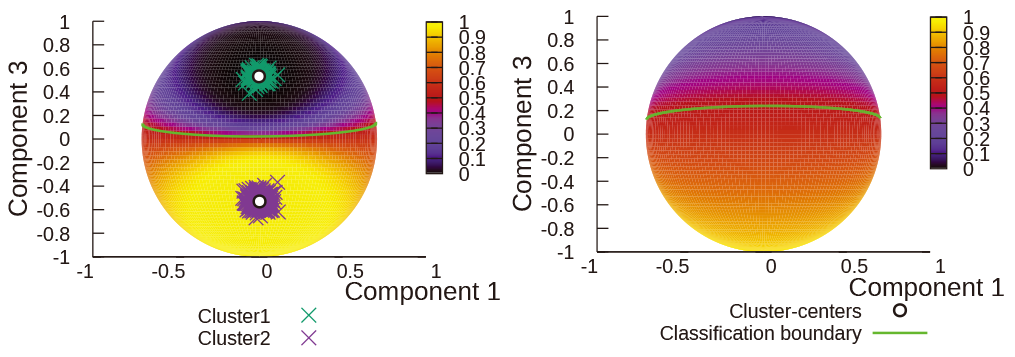
Fuzzy classification function of TYFCD
1. Introduction
Clustering partitions a dataset into subsets known as clusters. Objects assigned to the same cluster exhibit greater similarity than those assigned to different clusters. In a fuzzy clustering framework, each object can belong to multiple clusters with varying degrees of membership. Fuzzy \(c\)-means (FCM) 1 is one of the most widely used fuzzy clustering algorithms for vectorial data. In this study, we refer to the original formulation as the standard FCM (SFCM) to distinguish it from variants such as Tsallis entropy-based FCM (TFCM) 2, which is obtained by introducing Tsallis entropy regularization into the SFCM objective function.
However, in many real-world datasets, directional information plays a more important role than magnitude. These data are naturally represented as spherical data on a unit hypersphere through normalization. This representation removes scale effects and enables similarity to be evaluated based on direction, which is particularly useful in high-dimensional settings such as document analysis. The direct application of clustering methods designed for Euclidean space may be inappropriate for such data.
To address this issue, Yang et al. 3 proposed the fuzzy \(c\)-directions (FCD), a fuzzy clustering method derived from the von Mises–Fisher (vMF) distribution, which is a canonical probability distribution on a unit hypersphere. In the same study, they further incorporated a similarity-based clustering method (SCM) to automatically determine the number of clusters and initial solutions, thereby forming a more comprehensive unsupervised clustering framework for spherical data. In this study, we refer to the vMF-based formulation as Yang-type fuzzy \(c\)-directions (YFCD).
Although the automatic determination of cluster numbers and initializations is certainly important in unsupervised clustering, the applicability of the underlying clustering model itself becomes increasingly critical when dealing with extremely high-dimensional spherical data such as document datasets, the dimensionality of which may reach several thousand or tens of thousands. In such settings, the YFCD objective function may produce negative dissimilarity values because the vMF-based term includes logarithmic normalization constants and inner products, whose balance changes with dimensionality and concentration parameters. When such negative values occur, the membership updating rule of YFCD involves raising the possibly negative quantities to real-valued powers, which leads to undefined values in real space. Consequently, the algorithm may fail numerically or converge to degenerate cluster structures. This instability originates not from the implementation details but from the structural form of the YFCD objective function.
From this perspective, improving the intrinsic stability of the membership function becomes fundamental. We observed that introducing Tsallis entropy regularization provided a structural remedy to this problem. Tsallis entropy regularization introduces an additive offset into the effective dissimilarity that appears in the membership update. This can be interpreted as a stabilizing potential that compensates for the negative contributions arising from the vMF-based distance and the log-cluster size term. Consequently, the argument of the power function in the membership update can be maintained as non-negative under appropriate parameter settings, which ensures that the membership values remain well-defined in the real domain. Thus, Tsallis regularization plays a dual role: it increases the flexibility of fuzzification and simultaneously provides a mathematical mechanism that mitigates the degeneracy caused by negative effective distances.
Motivated by this observation, we focused on enhancing the intrinsic robustness of YFCD rather than on automatic model selection. We proposed a novel fuzzy clustering algorithm for spherical data, which is referred to as Tsallis entropy-regularized YFCD (TYFCD). The proposed method introduces Tsallis entropy regularization into the objective function of YFCD to stabilize membership estimation and improve robustness, particularly in high-dimensional scenarios. We also analyzed a limiting variant, referred to as TYFCD (\(m\to1\)), to clarify parameter roles.
First, we clarified the roles of the fuzzification parameters in the proposed method through numerical experiments on low-dimensional artificial datasets. We then evaluated its behavior on high-dimensional artificial datasets, demonstrating that TYFCD exhibited improved robustness under conditions such as low concentration parameters and imbalanced cluster sizes. Finally, experiments on 12 real datasets demonstrated that TYFCD consistently achieves higher clustering accuracy than existing approaches.
The remainder of this paper is organized as follows. Conventional clustering algorithms are introduced in Section 2. In Section 3, the proposed TYFCD method is described. Section 4 details the results of numerical experiments conducted to validate the effectiveness of the proposed algorithm. Finally, the conclusions are presented in Section 5.
2. Preliminaries
2.1. Entropy
The Shannon entropy \(H_{\mathsf{Shannon}}\) for a distribution \(P\) is defined as
2.2. Conventional Fuzzy Clustering Algorithms for Vectorial Data
Let \(X=\{x_k \in \mathbb{R}^M \mid k \in \{1,\dots,N\}\}\) be the dataset of \(M\)-dimensional points. The membership of \(x_{k}\) that belongs to the \(i\)-th cluster is denoted by \(u_{i,k}\) (\(i\in\{1,\dots,C\}, k\in\{1,\dots,N\}\)) and the set of \(u_{i,k}\) is denoted by \(u\), which is constrained with
In the SFCM and TFCM algorithms, the dissimilarity between object \(\#k\) and cluster \(\#i\) is defined as \(d_{i,k}^{(\mathsf{FCM})}=\|x_k-v_i\|_2^2\). These algorithms are based on the following optimization problems
2.3. Fuzzy Clustering Algorithms Based on vMF Distribution
Let \(X=\{x_{k}\in \mathbb{R}^{M}|\|x_k\|_2 =1, k\in\{1,\dots,N\}\}\) be a set of \((M-1)\)-dimensional spherical data points. The cluster center set is denoted by \(v=\{v_i\in\mathbb{R}^{M},~i\in\{1,\dots,C\}\}\), and the following constraint holds:
The YFCD 3 algorithm is based on the vMF distribution and is obtained using the following optimization problem:
Algorithm 1 (YFCD).
-
STEP 1.
Set the cluster number \(C\) and fuzzification parameters \(\lambda>0\) and \(m>1\). Initialize the membership \(u\) and cluster size controllers \(\alpha\).
-
STEP 2.Update \(v\) as follows:\begin{align} v_{i}=\dfrac{\displaystyle \sum_{k=1}^{N} \left(u_{i, k}\right)^m x_{k}}{\displaystyle \left\|\sum_{k=1}^{N} \left(u_{i, k}\right)^m x_{k}\right\|_{2}} \quad(i\in\{1,\dots,C\}). \label{eq:v-YFCD} \tag{12} \end{align}
-
STEP 3.Update \(\kappa\) by solving\begin{align} \dfrac{\displaystyle I_\frac{M}{2}(\kappa_i)}{\displaystyle I_{\frac{M}{2}-1}(\kappa_i)}&= \dfrac{\displaystyle \sum_{k=1}^N \left(u_{i,k}\right)^mx_k^\top v_i}{\displaystyle \sum_{k=1}^N \left(u_{i,k}\right)^m} \notag\\ &\quad(i\in\{1,\dots,C\}), \label{eq:kappa-YFCD} \tag{13} \end{align}numerically.
-
STEP 4.
Update \(d_{i, k}^{(\mathsf{FCD})}\) using Eq. (10).
-
STEP 5.Update \(\alpha\) as follows:\begin{align} \alpha_i&=\left[ \sum_{j=1}^C \left( \frac{\displaystyle \sum_{k=1}^N \left(u_{j, k}\right)^m}{\displaystyle \sum_{k=1}^N \left(u_{i, k}\right)^m} \right)^{\vphantom{\frac{\sum}{\sum}}} \right]^{-1} \notag\\ &\quad(i\in\{1,\dots,C\}). \label{eq:alpha-YFCD} \tag{14} \end{align}
-
STEP 6.Update \(u\) as follows:\begin{align} u_{i,k}&=\frac{\left(\lambda d_{i,k}^{(\mathsf{FCD})}-\ln\left(\alpha_i\right)\right)^{\frac{1}{1-m}}} {\displaystyle \sum_{j=1}^{C}\left(\lambda d_{j,k}^{(\mathsf{FCD})}-\ln\left(\alpha_j\right)\right)^{\frac{1}{1-m}}}\notag\\ \label{eq:u-YFCD} &\quad(i\in\{1,\dots,C\},~k\in\{1,\dots,N\}). \tag{15} \end{align}
-
STEP 7.
Check the limiting criterion for \((u, v,\alpha, \kappa)\). If the criterion is not satisfied, return to 2.
Eq. (13) was solved using the approximation method proposed in 6 and refined by two Newton iterations, as follows 7. The initial value is given by
3. Proposed Algorithm
3.1. TYFCD
We propose the TYFCD algorithm. Because TFCM exhibited better classification accuracy than SFCM after Tsallis entropy regularization was applied, we constructed an optimization problem by adding a Tsallis entropy regularization term to YFCD. The TYFCD optimization problem is expressed as follows:
The TYFCD algorithm is derived as follows. The Lagrange function \(L_{\operatorname*{TYFCD}}(u, v, \alpha, \kappa, \gamma, \zeta, \eta)\) is expressed as
Based on Eq. (19), the optimal cluster centers \(v\) can be determined using the Lagrange multiplier \(\zeta_i\), as follows:
According to Eq. (20), the optimal cluster size controllers \(\alpha\) are expressed using the Lagrange multiplier \(\eta\), as follows:
According to Eq. (21), the concentration parameters \(\kappa\) are determined by solving the following equation:
To further simplify Eq. (36), we use a standard recurrence differential relationship for the modified Bessel function of the first kind:
Based on the discussion, the proposed TYFCD algorithm can be summarized as follows:
Algorithm 2 (TYFCD).
-
STEP 1.
Set the cluster number \(C\) and the fuzzification parameters \(\lambda>0\), \(\lambda^{\prime}>0\), and \(m>1\). Initialize the membership \(u\) and cluster size controller \(\alpha\).
-
STEP 2.
Update \(v\) using Eq. (31).
-
STEP 3.
Update \(\kappa\) by solving Eq. (39) numerically.
-
STEP 4.
Update \(d_{i, k}^{(\mathsf{FCD})}\) using Eq. (10).
-
STEP 5.
Update \(\alpha\) using Eq. (34).
-
STEP 6.
Update \(u\) using Eq. (27).
-
STEP 7.
Check the limiting criterion for \((u, v,\alpha, \kappa)\). If the criterion is not satisfied, return to 2.
Eq. (39) was solved in the same manner as Eq. (13) in Algorithm 1.
3.2. Relation to YFCD
In the previous subsection, it was noted that TYFCD is a generalization of YFCD that use the objective functions of both algorithms. We observed that TYFCD is a generalization of YFCD at the level of their algorithms, as described below. By setting the fuzzification parameter as \(\lambda^{\prime} \to + \infty\), the membership equation presented in Eq. (27) can be expressed as follows:
The fuzzy classification function (FCF) 8 describes the degree to which any point in an object space is quintessentially attached to a cluster by broadening membership over the entire space. The FCF is useful for clarifying the features of fuzzy clustering methods 8. The FCF is denoted as \(u(x)=\{u_i(x) \in [0,1],i\in\{1,\dots,C\}\}\) with respect to a new object \(x\). The FCFs of YFCD and TYFCD are defined as solutions to the following optimization problems:
3.3. TYFCD (\(m\to{}1\))
When conducting real dataset experiments with TYFCD, as described in the following section, we observed that high clustering accuracy was frequently achieved when the fuzzification parameter \(m\) (\(>1\)) took very small values (\(m\simeq{}1\)). This observation raised the concern that, within TYFCD, the fuzzification parameter \(m\) may not contribute to improving the clustering performance; rather, the accuracy increases as \(m\) is made arbitrarily close to its lower bound. Moreover, maintaining \(m\) at such an extremely small value may reduce the number of parameters that must be tuned, given that the original TYFCD involves three fuzzification parameters. Motivated by this insight, we constructed and implemented a variant of TYFCD in which the fuzzification parameter satisfies \(m\to{}1\), hereafter referred to as TYFCD (\(m\to{}1\)), and compared its clustering performance with that of the original TYFCD. The algorithmic formulation of TYFCD (\(m\to{}1\)) is described in the following. By letting the parameter \(m\) in the TYFCD objective function presented in Eq. (16) approach one, we obtain the optimization problem of TYFCD (\(m\to{}1\)) as follows:
Algorithm 3 (TYFCD (\(\boldsymbol{m\to{}1}\))).
-
STEP 1.
Set the cluster number \(C\) and fuzzification parameters \(\lambda>0\) and \(\lambda^{\prime}>0\). Initialize the membership \(u\) and cluster size controller \(\alpha\).
-
STEP 2.Update \(v\) as follows:\begin{align} v_{i}= \frac{\displaystyle\sum_{k=1}^{N} u_{i, k} x_{k}}{\displaystyle\left\|\sum_{k=1}^{N} u_{i, k} x_{k}\right\|_{2}} \quad(i\in\{1,\dots,C\}). \label{eq:v_EKLFCD} \tag{48} \end{align}
-
STEP 3.Update \(\kappa\) by solving\begin{align} \frac{I_\frac{M}{2}\left(\kappa_i\right)}{I_{\frac{M}{2}-1}\left(\kappa_i\right)}&= \frac{\displaystyle\sum_{k=1}^N u_{i,k} x_k^\top v_i}{\displaystyle\sum_{k=1}^N u_{i,k}} &\quad(i\in\{1,\dots,C\}), \label{eq:kappa_EKLFCD} \tag{49} \end{align}numerically.
-
STEP 4.
Update \(d_{i, k}^{(\mathsf{FCD})}\) using Eq. (10).
-
STEP 5.Update \(\alpha\) as follows:\begin{align} &\alpha_i= \frac{\displaystyle\sum_{k=1}^N u_{i, k}}{N} \quad(i\in\{1,\dots,C\}).\label{eq:alpha_EKLFCD} \tag{50} \end{align}
-
STEP 6.Update \(u\) as follows:\begin{align} u_{i,k}&=\frac{\left(\alpha_{i}\right)^{\frac{\lambda^{\prime}}{\lambda}} \exp\left(-\lambda^{\prime}d_{i,k}^{(\mathsf{FCD})}\right)} {\displaystyle\sum_{j=1}^{C} \left(\alpha_{j}\right)^{\frac{\lambda^{\prime}}{\lambda}} \exp\left(-\lambda^{\prime}d_{j,k}^{(\mathsf{FCD})}\right)}\notag\\ &\quad(i\in\{1,\dots,C\},~k\in\{1,\dots,N\}).\label{eq:u_EKLFCD} \tag{51} \end{align}
-
STEP 7.
Check the limiting criterion for \((u, v,\alpha, \kappa)\). If the criterion is not satisfied, return to 2.
Similar to Algorithms 1 and 2, the concentration parameter \(\kappa_i\) in Algorithm 3 was computed using the approximation method of 6 followed by two Newton iterations according to 7. Specifically, the initial value was set as
4. Numerical Experiments
4.1. Individual Features of Parameters \(m\), \(\boldsymbol{\lambda}\), and \(\boldsymbol{\lambda^{\prime}}\)
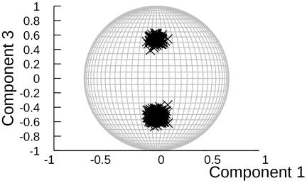
Fig. 1. Artificial dataset.
The features of Algorithm 2 and their relationships with Algorithm 1 were determined using the artificial data shown in Fig. 1. The dataset contained two clusters (\(C = 2\)) on a two-dimensional unit sphere and 100 of the 400 objects were generated using a vMF distribution with a mean of \(v_1 = (0, \sqrt{0.72}, \sqrt{0.28})^{\mathsf{T}}\) and concentration parameter \(\kappa_1 = 300.0\). The next 300 objects were also generated using a vMF distribution, but with a mean of \(v_2 = (0, \sqrt{0.72}, -\sqrt{0.28})^{\mathsf{T}}\) and concentration parameter \(\kappa_2 = 300.0\). Figs. 2–9 show the clustering results and FCF values for YFCD and TYFCD (subfigures (a) and (b) correspond to the front and back of the unit sphere, respectively), where the dark green crosses indicate cluster \(\#1\), the purple crosses denote cluster \(\#2\), and the outlined circles indicate cluster centers. The FCF values for the lower cluster, denoted as \(u_1(x)\), are visualized using a heatmap, in which high values are shown in yellow and low values are shown in black; the line for \(u_1(x) = u_2(x) = 0.5\), which represents the classification boundary, is indicated by the green line. Figs. 2 and 3 show the features of the YFCD fuzzification parameter \(m\). When the fuzzification parameter \(m\) increases, the FCF becomes fuzzy except near the cluster centers, and the classification boundaries remain largely unchanged. This feature is the same as that of the fuzzification parameter \(m\) in TYFCD. Figs. 2 and 4 show the features of the YFCD fuzzification parameter \(\lambda\). When the fuzzification parameter \(\lambda\) decreases, the FCF does not become fuzzy, but the classification boundary approaches the upper cluster, which has a smaller size. This feature is the same as that of the fuzzification parameter \(\lambda\) in TYFCD. Figs. 5 and 6 show the features of the TYFCD fuzzification parameter \(m\). Figs. 7 and 8 show the features of the TYFCD fuzzification parameter \(\lambda\). Figs. 5 and 9 show the features of the TYFCD fuzzification parameter \(\lambda^{\prime}\). When the fuzzification parameter \(\lambda^{\prime}\) decreases, the FCF becomes fuzzy near the classification boundary. Furthermore, the classification boundaries remain largely unchanged. Moreover, as \(\lambda^{\prime}\) approaches infinity, TYFCD approaches YFCD, as shown in Figs. 4 and 8. Therefore, TYFCD includes not only the features of YFCD but also new features.
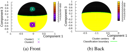
Fig. 2. YFCD: \((m,\lambda)=(1+10^{-15}, 0.0745)\).
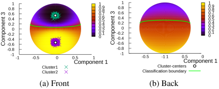
Fig. 3. YFCD: \((m,\lambda)=(1.4, 0.0745)\).
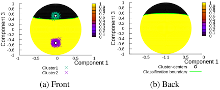
Fig. 4. YFCD: \((m,\lambda)=(1+10^{-15}, 0.009)\).
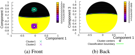
Fig. 5. TYFCD: \((m, \lambda, \lambda^{\prime})=(1+10^{-15}, 10^{4}, 0.6)\).
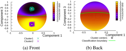
Fig. 6. TYFCD: \((m, \lambda, \lambda^{\prime})=(1.4, 10^{4}, 0.6)\).
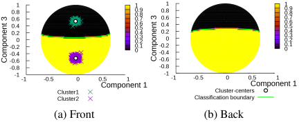
Fig. 7. TYFCD: \((m, \lambda, \lambda^{\prime})=(1+10^{-15}, 0.0745, 10^{4})\).
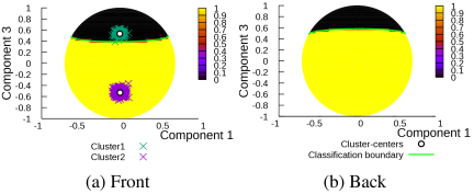
Fig. 8. TYFCD: \((m, \lambda, \lambda^{\prime})=(1+10^{-15}, 0.009, 10^{4})\).
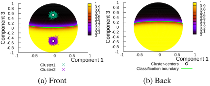
Fig. 9. TYFCD: \((m, \lambda, \lambda^{\prime})=(1+10^{-15}, 10^{4}, 0.06)\).
In summary, TYFCD involves three fuzzification-related parameters, namely \(m\), \(\lambda\), and \(\lambda'\), each of which plays a distinct role. The parameters \(m\) and \(\lambda\) correspond to those of YFCD. Specifically, \(m\) controls the overall degree of fuzziness throughout the object space except in the vicinity of cluster centers, whereas \(\lambda\) primarily determines the location of the decision boundary by controlling the influence of the cluster-size term relative to the vMF-based dissimilarity. By contrast, the newly introduced parameter \(\lambda'\) is unique to TYFCD. As observed in Figs. 5 and 9, decreasing \(\lambda'\) mainly increases fuzziness in the vicinity of the decision boundary while leaving the boundary location itself largely unchanged. Therefore, although both \(m\) and \(\lambda'\) contribute to fuzzification, their effects are qualitatively different: \(m\) controls global fuzzification over the object space, whereas \(\lambda'\) provides localized fuzzification around the decision boundary. This distinction provides an additional degree of freedom that is not available in YFCD. By independently adjusting \(m\) and \(\lambda'\), TYFCD can separately control global and boundary-specific fuzzification, thereby achieving more flexible membership distributions than YFCD. Furthermore, as \(\lambda'\to+\infty\), TYFCD reduces to YFCD, indicating that TYFCD generalizes the conventional framework while preserving it as a special case.
The purpose of this artificial dataset was not to evaluate the clustering accuracy under ambiguous conditions, but to visualize the influence of each parameter on the FCF and decision boundary. Because the FCF is evaluated over the entire data space, the behavior of the fuzzy memberships around the boundary regions can also be observed.
4.2. Performance Investigation Using High-Dimensional Artificial Datasets
4.2.1. Experimental Setup
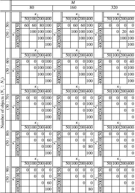
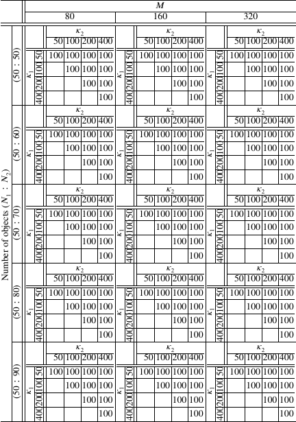
We conducted experiments using artificial datasets generated from the vMF distributions to investigate the behavior of the proposed method in high-dimensional settings. Each dataset consisted of two clusters, and the dimensionality, concentration parameters, and cluster size ratios were systematically varied to simulate different degrees of difficulty. The data dimension was varied among \(80\), \(160\), and \(320\). The cluster centers \(v_1\) and \(v_2\) were defined as follows: \(v_1\) had a value of \(1\) in the first dimension and \(0\) in all others, whereas \(v_2\) had a value of \(-1\) in the first dimension and \(0\) in all others. The numbers of objects in the first and second clusters of each dimension, denoted as \(N_1\) and \(N_2\), respectively, were set to \((N_1,N_2)\in\{(50,50)\), \((50,60)\), \((50,70)\), \((50,80)\), and \((50,90)\}\), corresponding to cluster size ratios of \(50:50\), \(50:60\), \(50:70\), \(50:80\), and \(50:90\), respectively. The concentration parameters of the vMF distribution, denoted as \(\kappa_1\) and \(\kappa_2\), were varied among \(50\), \(100\), \(200\), and \(400\). Five different artificial datasets were generated for each dimension, cluster size ratio, and concentration parameter combination.
The experimental settings were as follows. The fuzzification parameters were set to \(m\in\{1.0 + 10^{-15},1.0 +10^{-5},1.0+10^{-4},\dots,1.0+10^{0}\}\) and \(\lambda, \lambda'\in\{10^{-5},10^{-3},10^{-2},\dots,10^1\}\). The cluster size controllers were initialized to 1/2 and the membership degrees were initialized with five randomly selected distinct values. Among these runs, the solution with the lowest objective function value was selected. Whenever either algorithm converged to a feasible solution, the obtained clustering coincided perfectly with the ground-truth partition for the generated datasets. That is, successful runs always yielded perfect clustering accuracy. Consequently, the essential difference between the algorithms lies not in their ability to classify data correctly once convergence is achieved but in whether a valid solution can be obtained. However, under certain parameter configurations, the algorithms encountered numerical failures, such as the occurrence of NaN values or undefined membership updates, and thus failed to produce any clustering results. In such cases, the clustering accuracy can not be meaningfully evaluated because no valid partition is obtained. Therefore, instead of comparing the clustering accuracies, we evaluated the robustness of the algorithms. Specifically, we generated five datasets for each parameter setting and measured the proportion for which the algorithm successfully converged to a valid clustering result. Here, “success” means that the algorithm was completed without numerical failure and produced a clustering result identical to the ground truth. The success rates of YFCD and TYFCD are summarized in Tables 1 and 2, respectively. This measure reflects the numerical stability and practical reliability of the algorithms under the parameter settings considered.
4.2.2. Robustness Comparison Between YFCD and TYFCD
Table 1 shows that the robustness of YFCD deteriorates as the dimensionality increases, the concentration parameters decreases, or the cluster sizes become more imbalanced. We consider a case in which the data dimension is \(M=80\) and the cluster size ratio is \(50:50\). Under the conditions of \(\kappa_1 \ge 100\) and \(\kappa_2 \ge 100\), the success rate was \(100\) for all parameter settings, indicating a stable clustering performance. Moreover, even when \(\kappa_1=50\), the success rate reaches \(100\) if \(\kappa_2\) is sufficiently large, that is, \(\kappa_2=400\). However, the success rate decreased when either or both concentration parameters decreased. For example, the success rate remained at \(60\) when \(\kappa_1=\kappa_2=50\) reached \(80\), even for \((\kappa_1,\kappa_2)=(50,200)\). These results indicate that YFCD becomes unstable under low-concentration parameter settings. Focusing on the data dimension, the conditions under which a 100% success rate was achieved became increasingly restricted as the dimension increased. The success rate remained at \(100\) for \(M=160\) under the high-concentration parameter settings (\(\kappa_1 \ge 100\) and \(\kappa_2 \ge 100\)), whereas it decreased to zero when \(\kappa_1=\kappa_2=50\). A success rate of \(100\) was achieved for \(M=320\) only under high-concentration parameter settings (\(\kappa_1 \ge 200\) and \(\kappa_2 \ge 200\)). In particular, the success rate was zero regardless of the value of \(\kappa_2\) when \(\kappa_1=50\), and it was only \(20\) for \((\kappa_1,\kappa_2)=(100,200)\) and \(60\) for \((100,400)\) even when \(\kappa_1=100\). Moreover, the proportion of settings in which the computation was successfully completed decreased as the cluster size ratio became more imbalanced. When the cluster size ratio exceeded \(50:70\), computational failures became more frequent in the high-dimensional settings, except for a few cases with high-concentration parameters and low dimensionality. In particular, the algorithm failed to complete the computation under all experimental settings for \(M = 320\) and cluster size ratios of \(50:70\) or larger.
In contrast, Table 2 shows that the TYFCD computation was successfully completed and correct clustering results were obtained across all dimensions and cluster size settings under all considered experimental conditions. Notably, TYFCD consistently yielded perfect clustering results even in high-dimensional settings (\(M = 320\)) and under strongly imbalanced cluster size ratios such as \(50:90\). These results indicate that TYFCD exhibits high stability against both high dimensionality and cluster size imbalance.
4.2.3. Analysis of Numerical Instability
The instability observed in YFCD was not anticipated a priori but became evident through the above experiments. In particular, the low-dimensional experiments described in Section 4.1 indicated that decreasing the parameter \(\lambda\) systematically shifts the classification boundary toward smaller clusters. This behavior suggests that the balance among the vMF-based dissimilarity, cluster-size term, and fuzzification parameters plays a crucial role in determining the stability of membership updates. Next, we analyzed the structure of the membership-updating equation to clarify the mechanism behind this phenomenon.
Because the cluster size controller is less than one in YFCD, it follows that \(-\log(\alpha_i) > 0\). Moreover, as the dimensions increase and the concentration parameter decreases, \(d_{i,k}\) in Eq. (10) tends to decrease and can assume negative values. The vMF-based dissimilarities defined in Eq. (10) for dimension settings \(M = 80\), \(160\), and \(320\) and for concentration parameters up to \(\kappa = 400\) is illustrated in Fig. 10 for inner products \(x_k^\top v_i = 0.3\), \(0.6\), and \(0.9\), respectively. It can be confirmed from these figures that, as the dimensions increase, the object-cluster dissimilarity represented by Eq. (10) tends to decrease and becomes more likely to assume negative values. In contrast, the dependence on the concentration parameter exhibited a more intricate behavior. When \(x_k^\top v_i =0.3\), as shown in Fig. 10(a), a qualitative tendency was observed in which the dissimilarity decreased as the concentration parameter decreased. However, when \(x_k^\top v_i =0.6\), as shown in Fig. 10(b), the dissimilarity as a function of the concentration parameter exhibits a convex profile, which appears to increase as the concentration parameter decreases. Moreover, when \(x_k^\top v_i =0.9\), as shown in Fig. 10(c), the dissimilarity seemed to increase for smaller concentration values. This initially appeared to be inconsistent with the experimental results, in which a lower concentration parameter value yielded a negative dissimilarity value. To interpret this behavior, it should be noted that the vMF distribution became more dispersed as the concentration decreased. Therefore, objects that deviate substantially from the cluster center are more likely to appear, and the occurrence of objects with a relatively large inner product with the cluster center cannot be neglected in finite samples. Based on this observation, we infer that the YFCD algorithm becomes increasingly sensitive to the balance among the data dimension, concentration parameter, and inner product between objects and cluster centers under high-dimension and low-concentration conditions. Consequently, the cases in which the object-cluster dissimilarity defined by Eq. (10) becomes negative for at least one pair increase, leading to numerical instability.
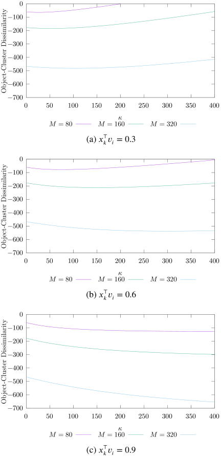
Fig. 10. Dissimilarity defined in Eq. (10) for different values of \(x_k^\top v_i\).
When \(d_{i,k}\) is negative and its absolute value is sufficiently large, the value \(\lambda d_{i,k} - \log(\alpha_i)\) can become negative depending on the values of \(\lambda\) and \(-\log(\alpha_i)\). In this case, the value of the YFCD membership update equation in Eq. (15), \((\lambda d_{i,k} - \log(\alpha_i))^{1/(1-m)}\), cannot be computed, and the algorithm cannot continue. This problem could be avoided by decreasing the fuzzification parameter \(\lambda\). Specifically, when setting \(\lambda\) to a sufficiently small value, the absolute value of \(\lambda d_{i,k}\) becomes smaller than that of \(-\log(\alpha_i)\), which causes the value \(\lambda d_{i,k} - \log(\alpha_i)\) to be positive. Consequently, \((\lambda d_{i,k} - \log(\alpha_i))^{1/(1-m)}\) becomes computable, which allows the algorithm to proceed. However, decreasing the value of \(\lambda\) causes the classification boundary to shift toward the cluster with a smaller cluster size (as observed in the previous subsection). If \(\lambda\) becomes excessively small, the classification boundary becomes excessively biased, resulting in all data points being assigned to a single cluster. In this case, the clustering result becomes invalid, and the cluster size controller converges such that one component corresponding to the cluster becomes one, whereas all others become zero. Subsequently, \(\log(\alpha_{i})\) for \(\alpha_i=0\) becomes undefined, and the algorithm cannot continue. In fact, in our experiments, when \(\lambda\) was set to a large value such as \(\lambda = 10\), the dissimilarity took negative values. As a representative example, we consider one of the two failure cases observed under an artificial dataset setting with \(M = 80\) and \((N_1:N_2) = 50:50\). When using the obtained concentration parameters \(\kappa_1 = 8.9946\) and \(\kappa_2 = 11.8881\), an inner product between an object and a cluster centers was \(x_{13}^\top v_1 = -0.0171\), and the dissimilarity was \(-65.4476\), which resulted in negative \((\lambda d_{i,k} - \log(\alpha_i))^{1/(1-m)}\) values. As another representative example, under the same experimental setting, when \(\lambda\) was set to an excessively small value such as \(\lambda = 10^{-7}\), the cluster size controller became crisp and the classification boundary was biased toward the cluster with a smaller cluster size. The cluster size controller corresponding to the cluster with index \(2\) had a value \(1\), indicating that the entire cluster size was assigned to a single cluster.
The proposed TYFCD resolves this issue as follows. When the dimension is excessively high and the concentration parameter is excessively low, \(d_{i,k}\) becomes negative and sufficiently large in magnitude, and thus, the term \(\lambda d_{i,k} - \log(\alpha_i)\) may again become negative depending on the values of \(\lambda\) and \(-\log(\alpha_i)\). However, by decreasing \(\lambda^{\prime}\) or \(m\), or selecting \(\lambda\) to be sufficiently small to prevent all components of the cluster size controller from becoming zero while avoiding excessive bias of the classification boundary, the value \(\lambda d_{i,k} - \log(\alpha_i) + \lambda / ((m-1)\lambda^{\prime})\) can be maintained as non-negative because the absolute value of \(\lambda / ((m-1)\lambda^{\prime})\) can be made sufficiently large compared with \(|\lambda d_{i,k} - \log(\alpha_i)|\). Consequently, the value used in the TYFCD membership updating equation, \((\lambda d_{i,k} - \log(\alpha_i) + \lambda / ((m-1)\lambda^{\prime}))^{1/(1-m)}\), can be computed, allowing the algorithm to continue.
These observations explain why TYFCD maintained stable convergence across all tested configurations, whereas YFCD frequently failed in high-dimensional or low-concentration settings.
4.2.4. Structural Difference Between YFCD and vMF Mixture Models
In the previous subsection, we discussed the numerical instability of YFCD mainly from the perspectives of high dimensionality, low concentration parameters, and cluster size imbalance. Another important aspect is the structural relationship between the vMF-based dissimilarity and the FCM-type power-based objective function.
In a standard vMF mixture model, membership-like posterior probabilities are derived directly from the likelihood function. Consequently, the vMF score is transformed using an exponential function, and negative values of the corresponding log-likelihood or dissimilarity do not directly lead to numerical difficulties. In contrast, YFCD incorporates vMF-based dissimilarity into the FCM framework, where the membership update is expressed using a power function. Therefore, when the effective dissimilarity term in the power function becomes negative, membership updates may become undefined in the real domain.
From this perspective, the numerical instability of YFCD can be interpreted as arising from the direct combination of vMF-based dissimilarity and power-type membership updates under certain conditions.
However, the FCM-type power structure itself plays an essential role in fuzzy clustering because it provides a simple and effective mechanism for controlling the degree of fuzziness. Many successful extensions of the FCM have been developed based on this framework. Therefore, entirely replacing the power-type update with an exponential-type update would eliminate one of the characteristic features of FCM-based approaches.
The proposed TYFCD preserves this FCM-type power structure while improving its compatibility with vMF-based dissimilarities through Tsallis entropy regularization. Specifically, the additional regularization term introduces a positive offset into the dissimilarity appearing in the membership update, thereby reducing the possibility of the argument of the power function becoming negative. Thus, TYFCD can be regarded as a method to mitigate the structural instability of YFCD while retaining the flexibility of the FCM-type fuzzification framework.
4.3. Clustering Accuracy Comparison Using Real Datasets
We compared the clustering accuracy of the proposed algorithm with that of conventional algorithms using 12 real datasets. The “Cora,” “WebKB,” and “CiteSeer” datasets are collections of scientific publications, each represented as a binary feature vector indicating the presence (1) or absence (0) of 1,432, 1,703, and 3,703 keywords, respectively. The documents in these datasets were categorized into seven, five, and six distinct topics, respectively 9. The remaining datasets were available from the CLUTO repository for clustering high-dimensional data 10. The “FBIS” dataset consists of document representations with 2,000 dimensions that are categorized into 17 distinct topics. It is based on Foreign Broadcast Information Service (FBIS) data labeled using TREC5 routing relevance judgments 11. The “ohscal” dataset, which is derived from the OHSUMED collection 12, consists of document representations with 11,465 dimensions that are categorized into 10 distinct topics. The “la1” dataset contains document representations with 29,714 dimensions and is derived from articles from the Los Angeles Times. The documents were categorized into six distinct topics: sports, metro, foreign, financial, national, and entertainment. The “la2” dataset also consists of document representations that are derived from articles from the Los Angeles Times. It contains 3,075 documents represented in 19,692 dimensions and categorized into the same six topics as in the la1 dataset. The “hitech” and “sports” datasets are based on news articles from the San Jose Mercury newspaper. The “hitech” dataset consists of document representations with 22,498 dimensions that are categorized into six distinct topics, whereas the “sports” dataset consists of document representations with 126,373 dimensions that are categorized into seven distinct topics. The “k1a” dataset was obtained from the WebACE project 13. It consists of 2,340 document objects represented in 21,839 dimensions that are categorized into 20 distinct topics. The “tr11” dataset consists of document representations with 6,429 dimensions that are categorized into nine classes: 1, 3, 4, 5, 6, 11, 12, 24, and 44. The “re0” dataset is derived from news articles in the Reuters-21,578 text categorization test collection (Distribution 1.0) 14 and consists of document representations with 2,886 dimensions. The dataset includes 13 categories. The number of objects, dimensions, classes, and objects in each class of these datasets are summarized in Table 3.
| Datasets | Data number | Dimension | Class |
Number of objects |
| in each class | ||||
| Cora | 2708 | 1432 | 7 | (818, 426, 418, 351, 298, 217, 180) |
| WebKB | 877 | 1703 | 5 | (415, 218, 125, 80, 39) |
| CiteSeer | 3312 | 3703 | 6 | (701, 668, 596, 590, 508, 249) |
| FBIS | 2463 | 2000 | 17 | (506, 387, 358, 190, 139, 125, 121, 119, 94, 92, 65, 48, 46, 46, 46, 43, 38) |
| ohscal | 11162 | 11465 | 10 | (1621, 1450, 1297, 1260, 1159, 1037, 1001, 864, 764, 709) |
| la1 | 3204 | 29714 | 6 | (943, 738, 555, 354, 341, 273) |
| la2 | 3075 | 19692 | 6 | (905, 759, 487, 375, 301, 248) |
| hitech | 2301 | 22498 | 6 | (603, 485, 481, 429, 187, 116) |
| sports | 8580 | 126373 | 7 | (3412, 23346, 1410, 809, 336, 145, 122) |
| k1a | 2340 | 21839 | 20 | (494, 278, 248, 187, 158, 142, 141, 125, 114, 74, 70, 65, 60, 54, 44, 24, 21, 18, 14, 9) |
| tr11 | 414 | 6429 | 9 | (132, 74, 69, 52, 29, 21, 20, 11, 6) |
| re0 | 1504 | 2886 | 13 | (608, 319, 219, 80, 60, 42, 39, 38, 37, 20, 16, 15, 11) |
The fuzzification parameters were varied based on the following rationale: experiments using artificial data revealed that a larger value of \(m\) yielded fuzzier clustering results, whereas a smaller value produced crisper results. If \(m\) becomes excessively large, the membership degrees approach \(1/C\) for all objects, causing all cluster centers to collapse to a single point and resulting in a meaningless clustering structure. Conversely, if \(m\) is set excessively small, the memberships become overly crisp, forcing objects near cluster boundaries, where fuzzy assignments are inherently appropriate, to be assigned values close to \(1\) or \(0\), thereby degrading clustering accuracy. Moreover, as noted previously, excessively small values of \(m\) can lead to numerical instability, eventually producing NaN values that prevent the algorithm from continuing. The fuzzification parameter \(\lambda\) also plays a critical role in both numerical stability and clustering behavior. \(\lambda\) affects the position of the classification boundary: if it is set too small, the classification boundary becomes excessively biased toward the cluster with a smaller cluster size, resulting in almost all data points being assigned to a single cluster. In such cases, the clustering result becomes invalid, and the cluster-size controller converges such that one component approaches one, whereas the others approach zero. Consequently, \(\log(\alpha_i)\) becomes undefined for \(\alpha_i = 0\), which prevents the algorithm from continuing. Similarly, a smaller value of \(\lambda^{\prime}\) yields fuzzier results, whereas a larger value produces crisper results. When \(\lambda^{\prime}\) is excessively small, the memberships again approach \(1/C\), causing all cluster centers to collapse and producing an uninformative clustering result. In contrast, if \(\lambda^{\prime}\) is excessively large, the memberships become overly crisp, leading to the same degradation in accuracy near the cluster boundaries. Furthermore, extremely large values of \(\lambda^{\prime}\) may cause a numerical overflow, making it impossible for the algorithm to proceed. Partition entropy (PE) can be used to detect a clustering results that are excessively fuzzy and meaningless 1. If the PE value associated with a result was equal to the logarithm of the number of clusters, the result was discarded because such a solution did not correspond to a meaningful clustering structure. Considering this phenomenon, we performed preliminary experiments to identify the parameter ranges that avoid overflow or NaN values and yield a PE value lower than \(\ln(C)\). We varied the parameter values as follows: \(m \in \{1.0 + 10^{-15}, 1.0 + 10^{-5}, 1.0 + 10^{-4}, 1.0 + 10^{-3}, 1.0 + 10^{-2}, 1.0 + 10^{-1}, 1.0 + 10^{0}\}\), \(\lambda \in \{10^{-5}, 10^{-3}, 10^{-1}, 1.0, 10, 100, 1000, 10000\}\), and \(\lambda^{\prime} \in \{10^{-5}, 10^{-3}, 10^{-1}, 1.0, 10, 100, 1000, 10000\}\). The number of clusters was set equal to the number of classes for each dataset. Each algorithm was run 10 times with each fuzzification parameter setting for a randomly selected initial membership, and the initial value of the cluster size controller was \(1/C\). The initial values of the concentration parameters \(\kappa\) were set according to the procedure described in 15. Iterative updates were terminated when the maximum absolute change in each component of the cluster centers, membership degrees, and concentration parameters fell below \(10^{-10}\). Results with the minimum objective function values were adopted. The clustering performance of the algorithms was evaluated using the adjusted Rand index (ARI) 16.
We attempted to apply YFCD to high-dimensional real datasets, as described previously. However, the computation failed for all the initializations and fuzzification parameter settings considered, and no valid results were obtained. This situation is analogous to that of the experiments detailed in Subsection 4.2, in which the dimensions of the real datasets were too high for YFCD. Therefore, we used a mixture of vMF distributions (movMF) 15, which is a representative clustering method for spherical data that generalizes spherical \(k\)-means 17, as a comparative method. As spherical \(k\)-means can be regarded as a limiting case of movMF, we focused on comparisons with movMF as a representative probabilistic baseline. In addition, we conducted experiments using TYFCD (\(m \to 1\)) to investigate the effect of the fuzzification parameter \(m\). Consequently, the real data experiments were carried out using three methods: movMF, TYFCD (\(m \to 1\)), and TYFCD.
| Dataset | vMF | TYFCD (\(m\to{}1\)) | TYFCD | |
| Cora | ARI | \(0.0829\) | \(\mathbf{0.1194}\) | \(\mathbf{0.1194}\) |
| PE | \(0.0013\) | \(0.1657\) | \(0.1641\) | |
| \(m\) | — | — | \(1.0+10^{-5}\) | |
| \(\lambda\) | — | \(1.0\) | \(1.0\) | |
| \(\lambda^{\prime}\) | — | \(0.1\) | \(0.1\) | |
| WebKB | ARI | \(0.1978\) | \(0.2149\) | \(\mathbf{0.2153}\) |
| PE | \(0.0002\) | \(0.0702\) | \(0.0652\) | |
| \(m\) | — | — | \(1.0+10^{-4}\) | |
| \(\lambda\) | — | \(1.0\) | \(100\) | |
| \(\lambda^{\prime}\) | — | \(0.1\) | \(0.1\) | |
| CiteSeer | ARI | \(0.1559\) | \(0.1612\) | \(\mathbf{0.1625}\) |
| PE | \(0.0003\) | \(0.0000\) | \(0.0000\) | |
| \(m\) | — | — | \(1.0+10^{-15}\) | |
| \(\lambda\) | — | \(1000\) | \(100\) | |
| \(\lambda^{\prime}\) | — | \(1000\) | \(100\) | |
| FBIS | ARI | \(0.2774\) | \(\mathbf{0.3540}\) | \(\mathbf{0.3540}\) |
| PE | \(0.0001\) | \(0.0000\) | \(0.0000\) | |
| \(m\) | — | — | \(1.0+10^{-15}\) | |
| \(\lambda\) | — | \(1.0\) | \(1.0\) | |
| \(\lambda^{\prime}\) | — | \(100\) | \(100\) | |
| ohscal | ARI | \(0.1764\) | \(\mathbf{0.1977}\) | \(\mathbf{0.1977}\) |
| PE | \(0.0001\) | \(0.0000\) | \(0.0000\) | |
| \(m\) | — | — | \(1.0+10^{-15}\) | |
| \(\lambda\) | — | \(100\) | \(100\) | |
| \(\lambda^{\prime}\) | — | \(1000\) | \(1000\) | |
| la1 | ARI | \(0.1107\) | \(0.1167\) | \(\mathbf{0.1170}\) |
| PE | \(0.0000\) | \(0.0000\) | \(0.0000\) | |
| \(m\) | — | — | \(1.0+10^{-15}\) | |
| \(\lambda\) | — | \(10\) | \(100\) | |
| \(\lambda^{\prime}\) | — | \(1000\) | \(1000\) | |
| la2 | ARI | \(0.1229\) | \(0.1259\) | \(\mathbf{0.1994}\) |
| PE | \(0.0000\) | \(0.0000\) | \(0.8214\) | |
| \(m\) | — | — | \(1.0+10^{-2}\) | |
| \(\lambda\) | — | \(1000\) | \(10\) | |
| \(\lambda^{\prime}\) | — | \(1000\) | \(0.001\) | |
| hitech | ARI | \(0.1719\) | \(\mathbf{0.1760}\) | \(\mathbf{0.1760}\) |
| PE | \(0.0000\) | \(0.0000\) | \(0.0000\) | |
| \(m\) | — | — | \(1.0+10^{-15}\) | |
| \(\lambda\) | — | \(100\) | \(100\) | |
| \(\lambda^{\prime}\) | — | \(100\) | \(100\) | |
| sports | ARI | \(0.1373\) | \(\mathbf{0.1398}\) | \(\mathbf{0.1398}\) |
| PE | \(0.0000\) | \(0.0000\) | \(0.0000\) | |
| \(m\) | — | — | \(1.0+10^{-15}\) | |
| \(\lambda\) | — | \(1.0\) | \(1.0\) | |
| \(\lambda^{\prime}\) | — | \(100\) | \(100\) | |
| k1a | ARI | \(0.3007\) | \(0.3363\) | \(\mathbf{0.3938}\) |
| PE | \(0.0000\) | \(0.0000\) | \(0.0000\) | |
| \(m\) | — | — | \(1.0+10^{-5}\) | |
| \(\lambda\) | — | \(10\) | \(10\) | |
| \(\lambda^{\prime}\) | — | \(1000\) | \(1.0\) | |
| tr11 | ARI | \(0.4277\) | \(0.4469\) | \(\mathbf{0.4561}\) |
| PE | \(0.0000\) | \(0.0005\) | \(0.0004\) | |
| \(m\) | — | — | \(1.0+10^{-5}\) | |
| \(\lambda\) | — | \(1.0\) | \(1.0\) | |
| \(\lambda^{\prime}\) | — | \(0.1\) | \(0.1\) | |
| re0 | ARI | \(0.1743\) | \(0.2290\) | \(\mathbf{0.2304}\) |
| PE | \(0.0000\) | \(0.0000\) | \(0.0001\) | |
| \(m\) | — | — | \(1.0+10^{-15}\) | |
| \(\lambda\) | — | \(0.1\) | \(0.1\) | |
| \(\lambda^{\prime}\) | — | \(1.0\) | \(1.0\) |
Table 4 presents the ARI values obtained using the three methods along with the corresponding PE values and parameter settings \((m, \lambda, \lambda^{\prime})\), under which these values were achieved for each dataset. The parameter values reported in Table 4 were selected using a grid search over predefined ranges, and the configuration that yielded the highest ARI was adopted for each dataset. The five rows for each dataset correspond to ARI, PE, \(m\), \(\lambda\), and \(\lambda^{\prime}\). As movMF does not use \(m\), \(\lambda\), or \(\lambda^{\prime}\), and TYFCD (\(m\to{}1\)) does not use \(m\), the entries that do not apply are marked with “—.” The three columns represent movMF, TYFCD (\(m\to{}1\)), and TYFCD, respectively, with the highest ARI value for each dataset highlighted in bold. The median ARI value of TYFCD was \(0.1986\), which was higher than those of the other algorithms: \(0.1731\) for movMF and \(0.1869\) for TYFCD (\(m\to{}1\)). The optimal fuzzification parameter \(m\) was \(1.0 + 10^{-15}\) for seven of the 12 datasets. At first glance, this value appears to be extremely close to \(1\), suggesting that fuzzification via \(m\) is ineffective. However, the ARI values obtained using TYFCD (\(m \to 1\)) were all equivalent to or lower than those of TYFCD. Furthermore, the median ARI value for TYFCD (\(m \to 1\)) did not exceed that for TYFCD. These results clearly show that even when the fuzzification parameter \(m\) is a value extremely close to \(1\), such as \(1.0 + 10^{-15}\), the behavior differs from that of TYFCD (\(m \to 1\)), where \(m \to 1\). The Wilcoxon signed-rank test with the Bonferroni correction for multiple comparisons confirmed the statistical significance of the differences (\(p = 0.0015\) and \(p = 0.0469\), respectively). Furthermore, the corresponding effect sizes were large (\(r>0.8\)), suggesting substantial improvement. These results indicate that TYFCD achieved a statistically significant improvement over movMF and TYFCD (\(m \to 1\)).
The experimental results showed that TYFCD achieved the highest clustering performance among the compared methods. From the comparison with TYFCD (\(m\to1\)), this improvement can be interpreted as resulting from the additional flexibility introduced by the parameter \(m\). On the other hand, from a practical perspective, it is also important to consider not only clustering accuracy but also the number of parameters that need to be tuned. TYFCD controls the three parameters \(m\), \(\lambda\), and \(\lambda'\), which enables more flexible adjustment of membership distributions but requires a larger parameter search cost. In contrast, TYFCD (\(m\to1\)) requires tuning only two parameters, \(\lambda\) and \(\lambda'\), and achieves a slightly lower accuracy with a lower parameter tuning cost. Therefore, the full TYFCD is preferable when maximizing clustering performance is the primary objective, whereas TYFCD (\(m\to1\)) can serve as a practical alternative when reducing parameter tuning cost is important. These two variants can be selected based on the trade-off between clustering accuracy and simplicity.
| Dataset | la1 | la2 | ||
| \(m\) | \(1+10^{-15}\) | \(1+10^{-2}\) | ||
| \(\lambda\) | 100 | 10 | ||
| Success times / ARI | \(\lambda'\) | \(10^{-5}\) | 10/0.0000 | 10/0.0000 |
| \(10^{-4}\) | 10/0.0000 | 10/0.0001 | ||
| \(10^{-3}\) | 10/0.0414 | 10/0.1994 | ||
| \(10^{-2}\) | 10/0.1170 | 0/– | ||
| \(10^{-1}\) | 10/0.1170 | 0/– | ||
| \(10^{0}\) | 10/0.1170 | 0/– | ||
| \(10^{3}\) | 10/0.1170 | 0/– | ||
| \(10^{5}\) | 10/0.1170 | 0/– | ||
| \(10^{6}\) | 10/0.1170 | 0/– | ||
| \(10^{7}\) | 0/– | 0/– | ||
| \(10^{9}\) | 0/– | 0/– | ||
Although TYFCD theoretically reduces to YFCD as \(\lambda'\to+\infty\), YFCD itself suffers from numerical instability on real high-dimensional datasets. Therefore, it is important to investigate how the numerical stability of TYFCD changes when \(\lambda'\) becomes sufficiently large.
To analyze this behavior, we conducted additional experiments using two representative datasets with different sensitivities to \(\lambda'\). Among the datasets used, “la1” achieved the highest ARI with the largest optimal value of \(\lambda'=10^3\), whereas “la2” achieved the highest ARI with the smallest optimal value of \(\lambda'=10^{-3}\). For each dataset, all parameters except \(\lambda'\) were fixed to those that achieved the highest ARI in the previous experiments. Specifically, \((m,\lambda)=(1+10^{-15},100)\) was used for “la1,” and \((m,\lambda)=(1+10^{-2},10)\) was used for “la2.”
The parameter \(\lambda'\) was varied over a wide logarithmic range, including both the values considered in the previous experiments and sufficiently large values beyond them: \(\lambda'\in{10^{-5},10^{-4},10^{-3},10^{-2},10^{-1}, 10^0,10^3,10^5,10^6,10^7,10^9}\). For each value of \(\lambda'\), ten random initializations were generated using the same procedure as in the previous experiments. The number of successful runs completed without numerical failures was recorded. When the algorithm successfully converged, the ARI corresponding to the minimum objective function value among ten trials was reported. The results are summarized in Table 5.
For the “la1” dataset, TYFCD successfully completed all ten trials for \(\lambda'=10^5\) and \(10^6\), which were larger than the previously examined values. Moreover, the best ARI was 0.1170, which is identical to that obtained for \(\lambda'=10^3\). However, when \(\lambda'\geq10^7\), numerical failure occurred for all initializations.
For the “la2” dataset, TYFCD achieved the highest ARI of 0.1994 at \(\lambda'=10^{-3}\), whereas a numerical failure occurred for all initializations when \(\lambda'\geq10^{-2}\). Thus, within the examined logarithmic grid, stable and unstable regions were clearly separated.
These results indicate that increasing \(\lambda'\) does not necessarily lead to a gradual degradation of clustering accuracy. Instead, TYFCD maintained numerical stability and the same clustering performance within a certain range of \(\lambda'\), whereas numerical instability appeared abruptly after \(\lambda'\) exceeded this range. This suggests that the transition toward a YFCD-like numerical behavior can appear as a sharp change in numerical stability rather than a gradual decrease in clustering accuracy.
It should be noted that the purpose of this supplementary experiment was not to estimate the exact critical value of \(\lambda'\). Because the transition point depends on the dataset, initialization, and other parameters, an exhaustive search for the exact threshold is beyond the scope of this study.
5. Conclusion
We proposed TYFCD, a Tsallis entropy-regularized fuzzy clustering algorithm based on the vMF distribution. Numerical experiments using artificial datasets demonstrated that the proposed algorithm generalizes the conventional YFCD and includes new characteristics. Moreover, experiments using high-dimensional artificial datasets confirmed that TYFCD exhibits high robustness against numerical instability, which is problematic for conventional methods with low-concentration parameters and highly imbalanced cluster sizes. In addition, experiments using 12 real datasets revealed that TYFCD achieves higher clustering accuracy than that of the mixture of vMF distributions and TYFCD \((m \to 1)\). These findings indicate that entropy-based regularization can serve not only as a fuzzification control method but also as a structural stabilization mechanism for spherical clustering.
In future work, we will extend this study in the following directions. We will consider applying SCM 3 to automatically determine the number of clusters and initial solutions, thereby forming a more comprehensive unsupervised clustering framework for high-dimensional spherical data. Although there is no theoretical or modeling requirement that forces the Tsallis entropy parameter \(q\) to be identified with the FCM fuzzification parameter \(m\), the Tsallis and FCM indices were aligned in this study to maintain analytical tractability, following the conventional formulation of TFCM. The issue of \(q\ne{}m\) will be addressed in future research.
- [1] J. C. Bezdek, “Pattern Recognition with Fuzzy Objective Function Algorithms,” Plenum Press, 1981. https://doi.org/10.1007/978-1-4757-0450-1
- [2] M. Ménard, V. Courboulay, and P.-A. Dardignac, “Possibilistic and probabilistic fuzzy clustering: Unification within the framework of the non-extensive thermostatistics,” Pattern Recognition, Vol.36, No.6, pp. 1325-1342, 2003. https://doi.org/10.1016/S0031-3203(02)00049-3
- [3] M.-S. Yang, S.-J. Chang-Chien, W.-L. Hung, “An unsupervised clustering algorithm for data on the unit hypersphere,” Applied Soft Computing, Vol.42, pp. 290-313, 2016. https://doi.org/10.1016/j.asoc.2015.12.037
- [4] H. Ichihashi, K. Honda, and N. Tani, “Gaussian Mixture PDF Approximation and Fuzzy c-Means Clustering with Entropy Regularization,” Proc. 4th Asian Fuzzy System Symp., pp. 217-221, 2000.
- [5] C. Tsallis, “Possible Generalization of Boltzmann-Gibbs Statistics,” J. Statist. Phys., Vol.52, Nos.1/2, pp. 479-487, 1988. https://doi.org/10.1007/BF01016429
- [6] I. S. Dhillon and S. Sra, “Modeling Data using Directional Distributions,” Technical Report TR-03-06, Department of Computer Sciences, The University of Texas at Austin, 2003.
- [7] S. Sra, “A Short Note on Parameter Approximation for von Mises–Fisher Distributions: And a Fast Implementation of Is(x),” Computational Statistics, Vol.27, No.1, pp. 177-190, 2012. https://doi.org/10.1007/s00180-011-0232-x
- [8] S. Miyamoto, H. Ichihashi, and K. Honda, “Algorithms for Fuzzy Clustering,” Springer, 2008. https://doi.org/10.1007/978-3-540-78737-2
- [9] LINQS Dataset. https://linqs.org/datasets/ [Accessed February 10, 2017]
- [10] G. Karypis, Karypis Lab, CLUTO - Software for Clustering High Dimensional Datasets. https://karypis.github.io/glaros/software/cluto/overview.html [Accessed February 8, 2017]
- [11] TREC: Text REtrieval Conf. Relevance Judgments. https://trec.nist.gov/data/qrels_eng/index.html [Accessed February 10, 2017]
- [12] W. Hersh, C. Buckley, T. J. Leone, and D. Hickam, “OHSUMED: an interactive retrieval evaluation and new large test collection for research,” Proc. of SIGIR94, pp. 192-201, 1994. https://doi.org/10.1007/978-1-4471-2099-5_20
- [13] D. Boley, M. Gini, R. Gross, E. H. Han, K. Hastings, G. Karypis, V. Kumar, B. Mobasher, and J. Moore, “Partitioning-based clustering for web document categorization,” Decision Support Systems, Vol.27, No.3, pp. 329-341, 1999. https://doi.org/10.1016/S0167-9236(99)00055-X
- [14] D. D. Lewis, “Reuters-21578 text categorization test collection distribution 1.0.” http://www.daviddlewis.com/resources/testcollections/reuters21578/ [Accessed December 1, 2025]
- [15] K. Hornik and B. Grün, “movMF: An R Package for Fitting Mixtures of von Mises-Fisher Distributions,” J. of Statistical Software, Vol.58, No.10, pp. 1-31, 2014. https://doi.org/10.18637/jss.v058.i10
- [16] L. Hubert and P. Arabie, “Comparing Partitions,” J. of Classification, Vol.2, pp. 193-218, 1985. https://doi.org/10.1007/BF01908075
- [17] I. S. Dhillon and D. S. Modha, “Concept Decompositions for Large Sparse Text Data Using Clustering,” Machine Learning, Vol.42, No.1, pp. 143-175, 2001. https://doi.org/10.1023/A:1007612920971
This article is published under a Creative Commons Attribution-NoDerivatives 4.0 Internationa License.