
Research Paper:
Adversarial Malware Detection Using Feature Contribution Difference Analysis with Kernel SHAP
Yoshiki Namura*, Tomotaka Kimura*,†
 , Moto Kamiura**
, and Jun Cheng*
*Graduate School of Science and Engineering, Doshisha University
1-3 Tataramiyakodani, Kyotanabe, Kyoto 610-0394, Japan
†Corresponding author
**Institute for Advanced Research and Education, Doshisha University
1-3 Tataramiyakodani, Kyotanabe, Kyoto 610-0394, Japan

Adversarial malware evades machine-learning-based detection by modifying its feature vector while preserving its malicious functionality. As attack methods continue to diversify, learning all possible adversarial patterns using conventional adversarial training has become impractical. However, because adversarial malware must retain its malicious functionality, certain intrinsic characteristics are common across diverse attacks. Based on this observation, we propose a two-stage adversarial malware detection method that leverages explainable artificial intelligence to analyze feature contributions in the prediction process. In the first stage, a neural network classifier performs the initial detection. In the second stage, Kernel SHAP is used to quantify each feature’s contribution to the model’s prediction, and the average contribution difference between benign software and malware is computed. The proposed method assigns higher weights to features with small contribution differences, which tend to exhibit high contributions when malware is present, and computes a maliciousness score to redetect adversarial samples that are misclassified as benign. Experimental results on Android application datasets demonstrate that the proposed method significantly outperforms existing approaches across four representative adversarial attacks (fast gradient sign method, JSMA, Mimicry, and Pointwise) without explicitly learning attack-specific characteristics.
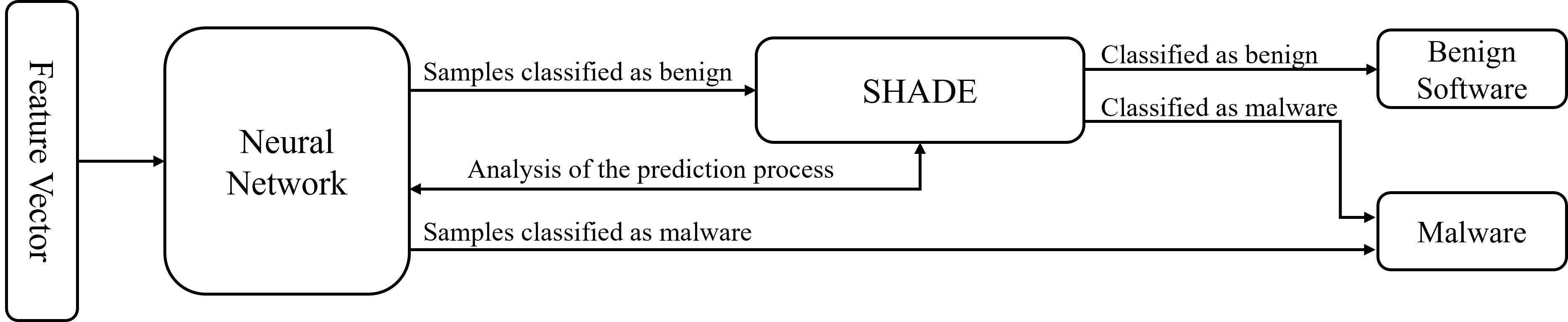
Detecting adversarial malware via SHADE
1. Introduction
In recent years, the damage caused by malware has increased significantly, including the theft of confidential information and the disruption of computer systems 1. Machine-learning-based malware detection has been widely studied to counter these threats 2,3. In this approach, feature representations extracted from malware and benign software are used to train a classification model that determines whether a given software sample is benign or malicious. Compared with traditional signature-based or rule-based methods, machine-learning-based approaches have been shown to achieve superior detection performance, particularly against previously unseen malware 4,5.
Despite this promise, machine-learning-based detection systems are vulnerable to adversarial malware 6. Adversarial malware is crafted to be misclassified as benign by modifying its feature representation such that the resulting feature vector crosses the decision boundary of the model while retaining its original malicious functionality. As adversarial malware generation techniques have become increasingly diverse in recent years, it has become impractical to comprehensively learn all possible attack patterns using conventional adversarial training alone 7. This has motivated the need for detection approaches that do not rely on explicitly learning each attack strategy.
To address this challenge, we observe that adversarial malware must preserve its malicious functionality regardless of the attack method used 8. This constraint implies that certain intrinsic malware characteristics remain in the prediction process, even after adversarial modification. Based on this insight, this study employs explainable artificial intelligence (XAI) to analyze the prediction process of machine-learning-based detection systems and to identify software that retains malware-specific characteristics in its feature contributions.
The proposed method adopts a two-stage detection framework. In the first stage, a neural network (NN) classifier performs an initial binary classification. In the second stage, samples classified as benign are reexamined using Kernel SHAP (SHapley Additive exPlanations), a representative XAI technique that quantifies the contribution of each input feature to the model’s prediction 9. By computing the average contribution difference between benign software and malware and evaluating whether the contribution pattern of a given sample is consistent with benign behavior, the method redetects adversarial malware that evades the first-stage classifier.
This study extends our previous work 10. In the conference version, we computed the average feature contributions from a mixed dataset containing both benign software and malware and used the resulting contribution ranking as weights to detect adversarial malware. However, this approach does not distinguish between features that contribute to benign classification and those that contribute to malware classification, thereby limiting its ability to capture malware-specific characteristics. In this extended version, we compute the average feature contributions for benign software and malware separately and introduce their differences as a new indicator. By focusing on features with small contribution differences that tend to retain high contributions when malware is present, the proposed method achieves more principled and effective detection. We also provide a more detailed description of the detection mechanism, expand the experimental evaluation with additional attack methods, present a fair comparison under equivalent benign-class accuracy, and analyze the feature contribution patterns and threshold sensitivity to demonstrate the robustness of the proposed approach.
The main contributions of this paper are summarized as follows:
-
・
We propose the concept of average contribution difference, which is computed by separately deriving the average feature contributions for benign software and malware using Kernel SHAP and taking their element-wise differences. This indicator enables the identification of features that retain malware-specific contribution patterns, regardless of adversarial modifications.
-
・
We design SHADE (Shapley-based Adversarial Malware Detection Enhancement), a second-stage detector that assigns higher weights to features with small contribution differences and computes a maliciousness score to redetect adversarial malware misclassified as benign by the first-stage classifier.
-
・
We conduct comprehensive experiments on four representative adversarial attacks (fast gradient sign method (FGSM), JSMA, Mimicry, and Pointwise) and demonstrate that the proposed method significantly outperforms existing approaches, including adversarial-training-based methods. We also analyze the feature contribution patterns and threshold sensitivity and conduct a fair comparison under equivalent benign-class accuracy to validate the robustness of the proposed approach.
The remainder of this paper is organized as follows: Section 2 reviews malware and adversarial malware detection. Section 3 describes the proposed method. Section 4 presents the experimental evaluation and discusses the results. Finally, Section 5 concludes the study.
2. Malware Detection and Adversarial Malware
2.1. Machine-Learning-Based Malware Detection
Malware detection aims at determining whether a software sample is malicious or benign 11. In recent years, machine-learning-based approaches have been widely adopted for this purpose, as they can be generalized to previously unseen malware variants.
In machine-learning-based malware detection, the behavioral or structural characteristics of the software are extracted and encoded as feature vectors. A classifier then takes these vectors as input and determines whether the software exhibits characteristics indicative of malware.
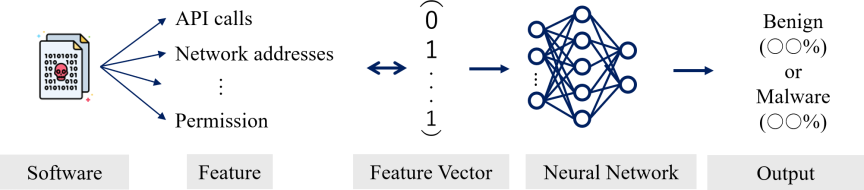
Fig. 1. Overview of NN-based malware detection.
Figure 1 illustrates a NN-based malware detection system. Given an input feature vector, the classifier outputs the probability that the software is benign and the probability that it is malware. Software is classified as malware when the malware probability exceeds the benign probability.
A commonly used feature representation is a binary vector based on API calls 12, where each element indicates whether a specific API is invoked during program execution.
Previous studies demonstrated the effectiveness of this approach. For example, 13 constructed a detection system using both dynamic and static analysis features and evaluated several models, including gradient boosting trees, random forests, and decision trees, reporting a detection accuracy of approximately 99% on Windows PE files. Similarly, 14 proposed a system based on memory and system behavior features using random forest and naïve Bayes classifiers, achieving an accuracy exceeding 99%.
2.2. Adversarial Malware
Adversarial malware refers to malicious software that has been intentionally modified to evade detection using machine-learning-based malware detection systems. By manipulating certain features, adversarial malware can cause the detection system to misclassify malware as benign software while preserving its malicious functionality. Because such attacks increase the risk of false negatives, the development of detection systems that are robust against adversarial manipulation has become an important challenge in malware analysis.
| Feature sets | 0 \(\rightarrow\) 1 | 1 \(\rightarrow\) 0 | |
| Manifest | Hardware | \(✓\) | \(\times\) |
| Requested permissions | \(✓\) | \(\times\) | |
| Application components | \(✓\) | \(✓\) | |
| Intents | \(✓\) | \(\times\) | |
| DexCode | Restricted API calls | \(✓\) | \(✓\) |
| Used permission | \(\times\) | \(\times\) | |
| Suspicious API calls | \(✓\) | \(✓\) | |
| Network addresses | \(✓\) | \(✓\) | |
2.2.1. Constraints on Feature Modification
Feature manipulation in adversarial malware generation cannot be performed arbitrarily, and modifications must satisfy certain constraints to preserve the malicious functionality of the software.
Table 1 summarizes the constraints on the Android software features 8. For each feature category, the table indicates whether adding a feature (0 \(\rightarrow\) 1) or removing a feature (1 \(\rightarrow\) 0) is permitted without breaking malware functionality.
2.2.2. Attack Methods
Adversarial attacks against malware detection systems are generally categorized as white-box or black-box attacks.
White-box attacks assume that the attacker has full knowledge of the target model, including its architecture and parameters 15. Based on this information, attackers generate perturbations that manipulate feature vectors to induce misclassification.
A representative white-box attack method is the FGSM 16, which generates adversarial examples using the gradient information of the target model.
By contrast, black-box attacks assume that the attacker has access only to the input–output behavior of the target model 15. The attackers repeatedly query the model and modify the feature vector based on the observed outputs.
Mimicry attacks 8,17 are typical examples of black-box attacks in which malware features are modified to resemble those of benign software while satisfying feature manipulation constraints. Such attacks are flexible because they require no internal information regarding the target model.
2.3. Related Work on Adversarial Malware Detection
To defend against adversarial malware, adversarial training has been widely studied 18,19. In this approach, adversarial malware samples generated by attack algorithms are incorporated into the training data such that the detection model learns to recognize adversarial feature patterns, thereby improving its robustness against known attack strategies.
The general procedure of adversarial training is as follows.
-
1.
Train an initial detection model using a benign software dataset and a malware dataset.
-
2.
Generate adversarial malware samples by applying adversarial attacks to the initial model.
-
3.
Combine the original training data with the generated adversarial samples to form an augmented training set.
-
4.
Retrain the detection model using the augmented training set.
The models retrained in this manner can achieve improved robustness against the types of adversarial malware included in the augmented training set. However, machine-learning models have a limited capacity to accommodate an ever-growing number of adversarial patterns 20, and as attack methods continue to diversify, it becomes increasingly difficult to learn all possible adversarial malware variants comprehensively.
Several studies have attempted to address this limitation using improved adversarial training strategies. For example, 21 proposed a reinforcement-learning-based approach that generates adversarial malware using Q-learning and retrains the detection system using the generated samples. 22 introduced principled adversarial malware detection, which improves robustness by learning diverse adversarial patterns through adversarial training. Although these methods enhance the detection performance against specific attack types, they remain fundamentally limited by their reliance on explicitly learning adversarial patterns, which makes it difficult to generalize them to unseen or novel attacks.
An alternative is to leverage XAI techniques to analyze the prediction process and detect anomalies in feature contributions. In our previous work 10, we proposed Mixed-SHAP, which applies Kernel SHAP to a mixed dataset of benign software and malware to compute average feature contributions and uses contribution-based ranking for detection. However, this approach does not distinguish between benign-specific and malware-specific contribution patterns, which limits its effectiveness against attacks such as FGSM and Mimicry. In this study, we extend this line of research by computing contribution averages for benign and malware samples separately and introducing their differences as a more principled detection indicator, thereby achieving robust detection across diverse attack types without relying on adversarial training.
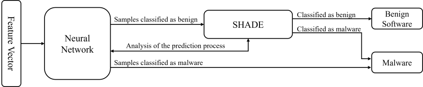
Fig. 2. Two-stage detection process.
3. Two-Stage Detection with SHADE
3.1. Overview
Figure 2 illustrates the overall structure of the proposed method, which consists of two stages: a NN that performs the initial classification and SHADE, which analyzes the prediction process to perform complementary detection.
In the first stage, the NN classifies the input feature vectors as benign software or malware. Because this classifier is vulnerable to adversarial malware and may misclassify malware as benign, the second stage introduces SHADE to revalidate the detection results. SHADE uses Kernel SHAP to compute feature contributions (i.e., the influence that each element of the feature vector exerts on the prediction). It then evaluates the quantitative differences in contribution trends between benign and malicious samples and assesses the consistency of explanations to redetect misclassified adversarial malware.
The key insight underlying SHADE is that benign software and malware exhibit systematic differences in their feature-contribution patterns. By leveraging this differential information, we can identify abnormal contribution patterns caused by adversarial manipulations, which are difficult to capture using conventional classifications alone.
Specifically, the training data are split into a benign dataset \(\mathcal{D}_B\) and a malware dataset \(\mathcal{D}_M\). Using Kernel SHAP, we compute the average contribution vectors \(\overline{\boldsymbol{{c}}}_B\) and \(\overline{\boldsymbol{{c}}}_M\) for benign classification in each dataset and derive the difference vector \(\overline{\boldsymbol{{c}}} = \overline{\boldsymbol{{c}}}_B - \overline{\boldsymbol{{c}}}_M\). Features with large differences reflect the properties of the benign software, whereas those with small differences retain malware-specific properties. The proposed method assigns higher weights to features with small differences during detection, thereby achieving high accuracy even against adversarial malware disguised as benign.
3.2. First Stage: Classification Using NNs
In the first stage, a NN performs a binary classification to determine whether the input binary feature vector represents benign software or malware. The classifier is trained using feature vectors of benign software and malware but does not include adversarial malware samples. Consequently, adversarial malware can evade the first-stage classifier by modifying its feature vector to resemble that of benign software.
To compensate for such misclassifications, samples classified as benign in the first stage are forwarded to the second-stage detector, SHADE, for re-evaluation. Samples classified as malware in the first stage are directly flagged as malicious, and no further analysis is performed.
3.3. Second Stage: SHADE
In the second stage, samples classified as benign in the first stage are re-evaluated from the perspective of prediction explainability. The SHADE detector analyzes the prediction process to identify misclassified adversarial malware. SHADE operates in two phases as illustrated in Figs. 3 and 4.
In the first phase, the Average Contribution Difference Calculation Phase, Kernel SHAP is applied to the training data to compute the Shapley values representing each feature’s contribution to benign classification for both benign and malware samples separately. The average contribution difference for each feature is derived by subtracting the average malware contribution from the average benign contribution. This difference quantitatively captures the disparity in how each feature influences the prediction of benign and malware samples. Features with a large average contribution difference tend to contribute strongly when the input is benign, whereas those with a small average contribution difference tend to contribute strongly when the input is malware.
In the second phase, the Detection Phase, Kernel SHAP is applied to the target sample. The resulting contribution vector is combined with the precalculated average contribution difference to assess whether the explanatory pattern of the sample is consistent with benign behavior. If features with small average contribution differences exhibit large contributions despite the sample being classified as benign, the inconsistency suggests the presence of malware, and the sample is reclassified accordingly.
3.3.1. Average Contribution Difference Calculation Phase
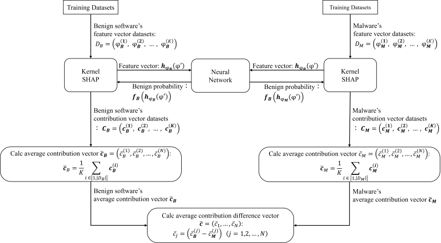
Fig. 3. Average contribution difference calculation phase.
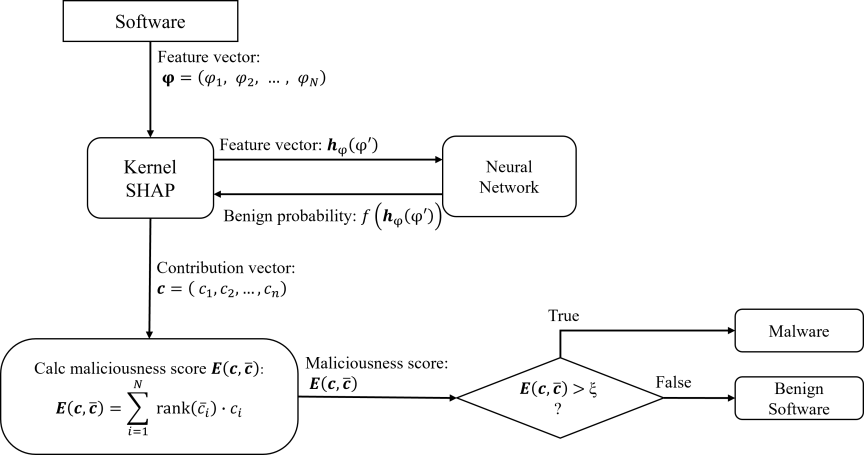
Fig. 4. Detection phase.
In this phase, Kernel SHAP is applied to the trained NN model \(f\) (as described in Section 3) using the training datasets \(\mathcal{D}_B\) (benign software) and \(\mathcal{D}_M\) (malware) to compute the average contribution difference for each feature. Let \(\boldsymbol{{\varphi_B}}^{(i)}\) and \(\boldsymbol{{\varphi_M}}^{(i)}\) denote the \(i\)-th feature vector in each dataset, where \(|\mathcal{D}_B|\) and \(|\mathcal{D}_M|\) denote the number of samples in each dataset. Let the complete set of feature vectors be \(\mathcal{F}=\{\boldsymbol{{\varphi_B}}^{(i)},\boldsymbol{{\varphi_M}}^{(i)} \mid i= 1, 2, \ldots, K\}\), where \(K = \max(|\mathcal{D}_B|, |\mathcal{D}_M|)\). Each feature vector is input into Kernel SHAP, which performs the optimization described below to obtain the contribution vector \(\boldsymbol{{c}}_B^{(i)}\) for benign software and \(\boldsymbol{{c}}_M^{(i)}\) for malware.
Kernel SHAP estimates the contribution of each feature to the prediction of a machine-learning model by constructing and optimizing a local linear surrogate model. For a feature vector \(\boldsymbol{{\varphi}} \in \mathcal{F}\), Kernel SHAP introduces a mask vector \(\boldsymbol{{\varphi}}^{\prime}\), an \(N\)-dimensional binary vector in which elements equal to 1 retain the corresponding feature and elements equal to 0 remove it. The masked feature vector is obtained via element-wise multiplication (\(\odot\)):
To derive the average contribution difference, we first compute the contribution vectors \(\boldsymbol{{c}}_B^{(i)}\) and \(\boldsymbol{{c}}_M^{(i)}\) for each feature vector, \(\boldsymbol{{\varphi}}_B^{(i)} \in \mathcal{D}_B\) and \(\boldsymbol{{\varphi}}_M^{(i)} \in \mathcal{D}_M\), respectively. The average contribution vectors \(\overline{\boldsymbol{{c}}}_B\) and \(\overline{\boldsymbol{{c}}}_M\) are computed as follows:
The average contribution difference vector \(\overline{\boldsymbol{{c}}}=(\overline{c}_1, \overline{c}_2, \ldots, \overline{c}_N)\) is then obtained by computing the element-wise difference.
3.3.2. Detection Phase
During the detection phase, the target software is represented by the feature vector \(\boldsymbol{{\varphi}}\), which is input into Kernel SHAP to obtain the feature contribution vector \(\boldsymbol{{c}} = (c_1, c_2, \dots, c_N)\) using the same procedure as in the previous phase.
As discussed above, features with small average contribution differences tend to exhibit larger contributions to malware than to benign software. Therefore, if a sample classified as benign in the first stage has large contributions concentrated on features with small contribution differences, this constitutes an inconsistency, suggesting that the sample may actually be malware.
To quantify this inconsistency, we compute the maliciousness score \(E(\boldsymbol{{c}}, \overline{\boldsymbol{{c}}})\) as the weighted sum of each feature’s contribution \(c_i\) and its corresponding rank \(\mathrm{rank}(\overline{c}_i)\):
4. Performance Evaluation
4.1. Experimental Settings
We evaluated the proposed method using the AndroZoo dataset 23, which is a large-scale repository of Android applications provided by the University of Luxembourg. From this dataset, 14,275 benign and 14,275 malware APK (Android Application Package) files were selected.
Following 8, we extracted the 100 most frequently occurring features from the training data and represented each sample as a 100-dimensional binary feature vector, where each element indicates the presence or absence of a specific feature.
The dataset was divided as follows: 60% for training, 20% for validation, and 20% for testing; 500 samples were selected as the test set. The average contribution difference was computed prior to testing, using 500 benign and 500 malware samples from the training data.
For each of the following four adversarial malware generation methods, 500 adversarial samples were generated:
-
FGSM:
A white-box attack that computes the gradients of the loss function with respect to the input features and applies perturbations in the gradient direction to maximize the loss 16.
-
JSMA:
A white-box attack that computes the Jacobian matrix of the model output with respect to the input features and greedily selects the most effective feature perturbations to induce misclassification with minimal modifications 24.
-
Mimicry:
A black-box attack that replaces malware features with those of benign software while retaining only the minimum features necessary for malicious functionality 17.
-
Pointwise:
A black-box attack that iteratively removes individual feature perturbations to minimize the total number of modified features while maintaining misclassification 8.
The NN used in the proposed method has a four-layer architecture with two hidden layers of 160 neurons each. Training was performed with a batch size of 128, 150 epochs, a learning rate of 0.001, ReLU activation, and Adam optimizer. The SHADE threshold was set to \(\xi = 16.7\).
The following detection systems were used as baselines for comparison:
-
ADE-MA [8]:
An adversarial-training-based detection system that uses an ensemble of five NNs, in which the average of each NN’s logit serves as the final output. Each NN has the same four-layer architecture as the proposed method (two hidden layers with 160 neurons, batch size of 128, 150 epochs, learning rate of 0.001, ReLU activation, and Adam optimizer). During training, four adversarial malware generation techniques (PGD-\(\ell_1\), PGD-\(\ell_2\), PGD-\(\ell_{\infty}\), and Adam-based FGSM) are employed. For each minibatch, the generation method that maximizes the loss function is selected, and the model is trained adversarially with the resulting samples.
-
Mixed-SHAP [10]:
A predecessor of the proposed method that applies Kernel SHAP to a mixed dataset containing both benign software and malware to compute a single average feature contribution vector \(\overline{\boldsymbol{{c}}}^{\mathrm{mix}}=(\overline{c}^{\mathrm{mix}}_1, \overline{c}^{\mathrm{mix}}_2, \ldots, \overline{c}^{\mathrm{mix}}_N)\). Using the same per-sample contribution vectors \(\boldsymbol{{c}}_B^{(i)}\) and \(\boldsymbol{{c}}_M^{(i)}\) defined in Section 3, the \(j\)-th element is given by:
\begin{align} \overline{c}^{\mathrm{mix}}_j &= \frac{1}{\left|\mathcal{D}_B\right|+\left|\mathcal{D}_M\right|} \left( \sum_{i=1}^{|\mathcal{D}_B|} c_{B,j}^{(i)} + \sum_{i=1}^{|\mathcal{D}_M|} c_{M,j}^{(i)} \right), \nonumber\\ & \qquad \left(j=1, 2, \ldots, N \right), \label{eq:mixed_shap} \tag{9} \end{align}where \(c_{B,j}^{(i)}\) and \(c_{M,j}^{(i)}\) denote the \(j\)-th elements of \(\boldsymbol{{c}}_B^{(i)}\) and \(\boldsymbol{{c}}_M^{(i)}\), respectively. Mixed-SHAP ranks features by \(\overline{c}^{\mathrm{mix}}_j\) in descending order and uses \(\mathrm{rank}(\overline{c}^{\mathrm{mix}}_j)\) as the weight in the maliciousness score in the same manner as the proposed method; if the weighted sum of contributions exceeds a threshold, the sample is classified as malware. Unlike the proposed method, which preserves class-specific information through the element-wise difference \(\overline{\boldsymbol{{c}}}=\overline{\boldsymbol{{c}}}_B-\overline{\boldsymbol{{c}}}_M\) in Eq. (7), Mixed-SHAP averages the benign and malware contributions over the mixed dataset (Eq. (9)), which partially cancels out class-specific tendencies because the benign and malware samples contribute to the benign probability in opposite directions. The NN configuration and training dataset are identical to those of the proposed method, with the threshold set to 18.0.
Because the performance is reported separately for each sample category, class-wise accuracy is defined as the proportion of samples in each category that are correctly classified. For benign software, this proportion corresponds to the true-negative rate (TNR). For conventional malware and each adversarial malware category (FGSM, JSMA, Mimicry, and Pointwise), it corresponds to the true-positive rate (TPR) of that category:
| Benign software | Malware | FGSM | JSMA | Mimicry | Pointwise | |
| Proposed method | 91.2 | 100.0 | 100.0 | 100.0 | 100.0 | 100.0 |
| Mixed-SHAP | 92.8 | 99.6 | 66.4 | 100.0 | 74.0 | 100.0 |
| NN | 98.6 | 97.1 | 1.0 | 18.6 | 0.0 | 0.0 |
| ADE-MA | 96.6 | 96.6 | 80.9 | 6.5 | 1.6 | 1.3 |
4.2. Evaluation Results
4.2.1. Comparison of Class-Wise Accuracy
Table 2 presents the class-wise accuracy [%] of each method. The proposed method achieves 100% class-wise accuracy against both conventional malware and all four types of adversarial malware, demonstrating that it successfully detects all the malicious samples without any false negatives.
Mixed-SHAP achieves 100% class-wise accuracy against JSMA and Pointwise attacks but suffers significant performance degradation against FGSM (66.4%) and Mimicry (74.0%) attacks. This suggests that for FGSM and Mimicry, averaging feature contributions over a mixed benign–malware dataset may obscure the differences between the benign and malware contribution patterns.
The baseline NN exhibits extremely low class-wise accuracy against all adversarial attacks, with 0% class-wise accuracy against both Mimicry and Pointwise attacks, indicating that the baseline NN is vulnerable to the four adversarial attacks evaluated in this study.
ADE-MA achieves reasonable class-wise accuracy against FGSM attacks (80.9%) owing to its adversarial training strategy; however, its performance declines sharply against JSMA (6.5%), Mimicry (1.6%), and Pointwise (1.3%) attacks. In this experiment, ADE-MA performed relatively well against FGSM but poorly against JSMA, Mimicry, and Pointwise attacks, suggesting that its robustness may depend on the similarity between the evaluated attacks and those used during training.
It should be noted that the proposed method exhibits slightly lower benign-class accuracy (91.2%) compared to the baseline NN (98.6%) and ADE-MA (96.6%). This trade-off arises because the second-stage SHADE detector reclassifies some benign samples as malware when their contribution patterns resemble those of malicious samples. To investigate whether this trade-off affects the fairness of the comparison, we conduct a controlled evaluation under equivalent benign-class accuracy in Section 4.2.4.
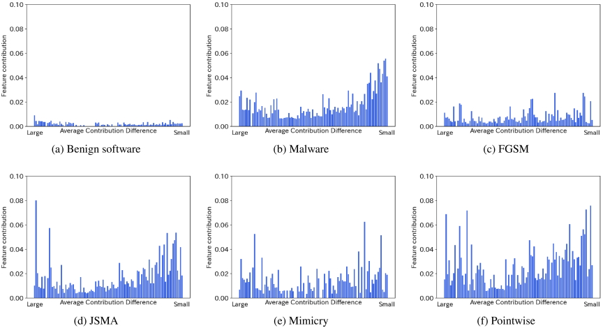
Fig. 5. Average contribution to the benign-probability output of the detection system.
4.2.2. Analysis of Feature Contribution Patterns
To better understand why the proposed method achieves robust detection across diverse attack types, we analyze the feature contribution patterns for each sample category. Fig. 5 shows the average feature contribution for each category, with features sorted in descending order of the average contribution difference from left to right.
For benign software, the contributions are uniformly low across all features, indicating that no individual feature dominates the prediction. By contrast, malware samples exhibit high contributions concentrated in features with small average contribution differences, confirming that malware-specific features play a dominant role in the prediction process.
For the adversarial malware, high contributions are observed for features with both large and small average contribution differences. This dual pattern reflects the effect of adversarial feature modifications: the original malware characteristics produce high contributions to features with small differences, whereas the added perturbations designed to induce misclassification increase the contributions to features with large differences.
Notably, the JSMA and Pointwise attacks exhibit contribution patterns similar to those of conventional malware. This is because these attacks aim to minimize the number of modified features, resulting in feature vectors that remain close to the original malware representation. In contrast, FGSM and Mimicry attacks show contribution patterns that partially resemble those of benign software because these methods do not constrain the number of modifications and thus produce feature vectors that diverge more substantially from the original malware.
Despite these variations in contribution patterns across attack types, the proposed method successfully detects all adversarial malware by focusing on the weighted contributions of features with small average contribution differences, which consistently reflect the presence of malicious functionality.
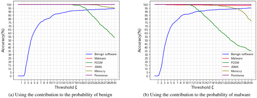
Fig. 6. Class-wise accuracy as a function of the threshold \(\xi\).
| Benign software | Malware | FGSM | JSMA | Mimicry | Pointwise | |
| Proposed method | 91.2 | 100.0 | 100.0 | 100.0 | 100.0 | 100.0 |
| NN-calibrated | 91.3 | 99.1 | 27.6 | 71.9 | 45.9 | 98.0 |
| ADE-MA-calibrated | 91.3 | 97.4 | 97.0 | 51.7 | 37.0 | 35.8 |
4.2.3. Sensitivity to Threshold
Figure 6 shows the class-wise accuracy as a function of the threshold \(\xi\), varied from 0 to 30. Fig. 6(a) presents the results using the contributions to the benign probability, and Fig. 6(b) presents the results using the contributions to the malware probability.
In both cases, the class-wise accuracy against FGSM attacks begins to decline as the threshold increases. This is attributable to the nature of FGSM, which leverages the full gradient information of the target model to modify features efficiently. The resulting contribution patterns closely resemble those of benign software, yielding lower maliciousness scores \(E\). This observation suggests that FGSM is the most challenging of the attacks evaluated against the proposed method. Nevertheless, at the chosen threshold of \(\xi = 16.7\), 100% class-wise accuracy is maintained across all evaluated attack types.
We next examine the relationship between the threshold and false positives using the benign software curve shown in Fig. 6(a). Because the benign software curve represents the TNR, a lower value corresponds to a higher false-positive rate. As \(\xi\) increases, the TNR rises monotonically because fewer benign samples exceed the threshold; at \(\xi=16.7\), the benign-class accuracy is \(91.2\%\). Lowering \(\xi\) can therefore increase the false-positive rate on benign software. Among the four evaluated attacks, the class-wise accuracy for FGSM is the first to decline as \(\xi\) increases, suggesting that FGSM imposes the tightest threshold constraint in this experiment. Mimicry remains at \(100\%\) until a substantially higher threshold is reached, whereas JSMA and Pointwise remain at \(100\%\) throughout the evaluated range. At the selected value \(\xi=16.7\), all four attack sets are detected at \(100\%\) class-wise accuracy, while the benign-class accuracy is \(91.2\%\). For the evaluated samples, lowering \(\xi\) below this value may increase false positives without improving attack detection, because the class-wise accuracy for every attack set is already \(100\%\); conversely, increasing \(\xi\) improves benign-class accuracy but begins to reduce the class-wise accuracy for FGSM. Thus, \(\xi=16.7\) provides a balance between false positives on benign software and false negatives on the evaluated attacks.
4.2.4. Fair Comparison Under Equivalent Benign-Class Accuracy
As discussed in Section 4.2.1, the proposed method exhibits a slightly lower benign-class accuracy (91.2%) than the baseline NN (98.6%) and ADE-MA (96.6%). A natural question arises: Does the superior adversarial detection of the proposed method simply result from a stricter decision threshold that sacrifices benign-class accuracy? To answer this question, we conduct a controlled evaluation with equivalent benign-class accuracies.
Specifically, we introduce two additional baselines:
-
NN-calibrated:
A variant of the baseline NN, whose decision boundary is adjusted such that its benign-class accuracy approximately matches that of the proposed method. This adjustment is performed by adding a constant \(1.0\times10^{-6}\) to the malware probability computed using the SoftMax function.
-
ADE-MA-calibrated:
A variant of ADE-MA with a similarly adjusted decision boundary. A constant of \(0.105\) was added to the benign probability computed using the SoftMax function to align its benign-class accuracy with that of the proposed method.
Table 3 presents the results of a fair comparison. All three methods operate with approximately 91% benign-class accuracy, allowing a direct comparison of the adversarial malware detection performance under the same trade-off condition.
Even when the benign-class accuracy is aligned at approximately 91%, the proposed method achieves 100% class-wise accuracy against all adversarial malware types, whereas both calibrated baselines exhibit significant performance gaps.
NN-calibrated shows a substantial improvement over the original NN (Table 2), particularly against Pointwise attacks (0.0% \(\rightarrow\) 98.0%) and JSMA attacks (18.6% \(\rightarrow\) 71.9%). However, it still fails to adequately detect FGSM (27.6%) and Mimicry (45.9%) attacks. This indicates that shifting the decision boundary improves the detection of some attack types, but does not fully compensate for the baseline classifier’s vulnerability in this experiment.
ADE-MA-calibrated achieves high class-wise accuracy against FGSM attacks (97.0%), benefiting from its adversarial training strategy. However, its performance against JSMA (51.7%), Mimicry (37.0%), and Pointwise (35.8%) attacks remains far below that of the proposed method. This result suggests that in the evaluated setting, adversarial training and decision boundary calibration do not yield uniformly high detection across the four attack methods.
These results demonstrate that the advantage of the proposed method is not a consequence of a strict decision threshold. Rather, the SHADE detector leverages fundamentally different information, namely feature contribution patterns derived from XAI analysis, which enables uniform detection across the four evaluated attack types under the matched benign-class accuracy considered in Table 3.
5. Conclusion
In this study, we propose a two-stage adversarial malware detection method that combines a NN classifier with SHADE, a second-stage detector that analyzes the prediction process using Kernel SHAP. By computing the average feature contribution difference between benign software and malware, the proposed method focuses on features that retain malware-specific characteristics and evaluates the consistency of explanations to redetect adversarial malware misclassified as benign. Experimental results using the AndroZoo dataset demonstrate that the proposed method significantly outperforms existing approaches in detecting adversarial malware generated by FGSM, JSMA, Mimicry, and Pointwise.
The key advantage of the proposed method is that it leverages the inherent differences in feature contribution patterns between benign software and malware, rather than explicitly learning adversarial attack patterns. The experimental results suggest that this approach may also have potential against unknown adversarial malware that retains malware-related functionality. However, this possibility remains to be experimentally validated.
Although the proposed method achieved high class-wise accuracy against adversarial malware, its benign-class accuracy decreased compared to that of the first-stage NN classifier alone. This is because the SHADE detector may misidentify benign samples whose feature contribution patterns deviate from the typical benign behavior. Improving the benign-class accuracy without sacrificing the adversarial malware detection performance is an important direction for future work.
In addition, the proposed method has a higher computational cost than that of the baseline methods. Because the second stage relies on Kernel SHAP, its per-sample cost is comparable to that of Mixed-SHAP, and both methods require substantially more computation than do NN and ADE-MA. The computational cost of Kernel SHAP remains a practical challenge. Because Kernel SHAP approximates Shapley values through iterative sampling of feature coalitions, the computation time increases with the number of features and samples to be analyzed. In real-time detection scenarios, this overhead may limit the applicability of the proposed method. Exploring more efficient explanatory methods, such as leveraging model-specific SHAP variants or reducing the number of coalitions required for a reliable approximation, is another important direction for future research. The second-stage cost may be reduced by decreasing the background size used by Kernel SHAP or by forwarding only low-confidence benign samples from the first stage; the resulting trade-off between computational cost and detection performance requires further evaluation.
Furthermore, differences in contributions observed in this study may have been influenced by the characteristics of the datasets used. In future work, we plan to evaluate the generalizability of the proposed method using different datasets and investigate its robustness against more sophisticated adversarial attacks. Finally, complementing the empirical results with a formal theoretical analysis of the maliciousness score, such as a characterization of the conditions under which functionality-preserving adversarial malware can be separated from benign software, is an important direction for future research.
- [1] A. P. Namanya, A. Cullen, I. U. Awan, and J. P. Disso, “The world of malware: An overview,” 2018 IEEE 6th Int. Conf. on Future Internet of Things and Cloud (FiCloud), pp. 420-427, 2018. https://doi.org/10.1109/ficloud.2018.00067
- [2] J. Singh and J. Singh, “A survey on machine learning-based malware detection in executable files,” J. of Systems Architecture, Vol.112, Article No.101861, 2021. https://doi.org/10.1016/j.sysarc.2020.101861
- [3] B. Yang, Y. Xiao, X. Wang, Z. Cui, and C. Peng, “An intrusion detection model based on afsa-svm for petroleum multi-channel industrial control network communication,” J. Adv. Comput. Intell. Intell. Inform., Vol.29, No.4, pp. 703-710, 2025. https://doi.org/10.20965/jaciii.2025.p0703
- [4] J. Saxe and K. Berlin, “Deep neural network based malware detection using two dimensional binary program features,” 2015 10th Int. Conf. on Malicious and Unwanted Software (MALWARE), pp. 11-20, 2015. https://doi.org/10.1109/malware.2015.7413680
- [5] D. Gibert, J. Planes, C. Mateu, and Q. Le, “Fusing feature engineering and deep learning: A case study for malware classification,” Expert Systems with Applications, Vol.207, Article No.117957, 2022. https://doi.org/10.1016/j.eswa.2022.117957
- [6] K. Grosse, N. Papernot, P. Manoharan, M. Backes, and P. McDaniel, “Adversarial examples for malware detection,” Lecture Notes in Computer Science, pp. 62-79, 2017. https://doi.org/10.1007/978-3-319-66399-9_4
- [7] G. Lan, Z. Gao, L. Tong, and T. Liu, “Class binarization to neuroevolution for multiclass classification,” Neural Computing and Applications, Vol.34, No.22, pp. 19845-19862, 2022. https://doi.org/10.1007/s00521-022-07525-6
- [8] D. Li and Q. Li, “Adversarial deep ensemble: Evasion attacks and defenses for malware detection,” IEEE Trans. on Information Forensics and Security, Vol.15, pp. 3886-3900, 2020. https://doi.org/10.1109/tifs.2020.3003571
- [9] S. M. Lundberg and S.-I. Lee, “A unified approach to interpreting model predictions,” Proc. of the 31st Int. Conf. on Neural Information Processing Systems, 2017.
- [10] Y. Namura, T. Kimura, M. Kamiura, and J. Cheng, “Adversarial malware detection using feature contribution analysis with Kernel SHAP,” Proc. of the 22nd Int. Conf. on Modeling Decisions for AI (MDAI’25), 2025.
- [11] I. A. Saeed, A. Selamat, and A. M. A. Abuagoub, “A survey on malware and malware detection systems,” Int. J. of Computer Applications, Vol.67, No.16, pp. 25-31, 2013. https://doi.org/10.5120/11480-7108
- [12] W. Yuan, H. H. Nguyen, L. Jiang, Y. Chen, J. Zhao, and H. Yu, “Api recommendation for event-driven android application development,” Information and Software Technology, Vol.107, pp. 30-47, 2019. https://doi.org/10.1016/j.infsof.2018.10.010
- [13] A. Hussain, M. Asif, M. B. Ahmad, T. Mahmood, and M. A. Raza, “Malware detection using machine learning algorithms for windows platform,” Lecture Notes in Networks and Systems, pp. 619-632, 2022. https://doi.org/10.1007/978-981-16-7618-5_53
- [14] A. Öztürk and S. Hızal, “Detection and analysis of malicious software using machine learning models,” Sakarya University J. of Computer and Information Sciences, Vol.7, No.2, pp. 264-276, 2024. https://doi.org/10.35377/saucis...1489237
- [15] C. Guo, J. Gardner, Y. You, A. G. Wilson, and K. Weinberger, “Simple black-box adversarial attacks,” Proc. of Int. Conf. on Machine Learning, pp. 2484-2493, 2019.
- [16] I. Goodfellow, J. Shlens, and C. Szegedy, “Explaining and harnessing adversarial examples,” Proc. of Int. Conf. on Learning Representations, 2015.
- [17] N. Srndic and P. Laskov, “Practical evasion of a learning-based classifier: A case study,” 2014 IEEE Symp. on Security and Privacy (SP), pp. 197-211, 2014. https://doi.org/10.1109/sp.2014.20
- [18] Y. Wang, X. Ma, J. Bailey, J. Yi, B. Zhou, and Q. Gu, “On the convergence and robustness of adversarial training,” Proc. of the 36th Int. Conf. on Machine Learning, pp. 6586-6595, 2019.
- [19] A. Shafahi, M. Najibi, M. A. Ghiasi, Z. Xu, J. Dickerson, C. Studer, L. S. Davis, G. Taylor, and T. Goldstein, “Adversarial training for free!” Advances in Neural Information Processing Systems, Vol.32, 2019.
- [20] F. Abramovich and M. Pensky, “Classification with many classes: Challenges and pluses,” J. of Multivariate Analysis, Vol.174, Article No.104536, 2019. https://doi.org/10.1016/j.jmva.2019.104536
- [21] H. Rathore, S. K. Sahay, P. Nikam, and M. Sewak, “Robust android malware detection system against adversarial attacks using Q-learning,” Information Systems Frontiers, Vol.23, No.4, pp. 867-882, 2021. https://doi.org/10.1007/s10796-020-10083-8
- [22] D. Li, S. Cui, Y. Li, J. Xu, F. Xiao, and S. Xu, “Pad: Towards principled adversarial malware detection against evasion attacks,” IEEE Trans. on Dependable and Secure Computing, Vol.21, No.2, pp. 920-936, 2024. https://doi.org/10.1109/tdsc.2023.3265665
- [23] K. Allix, T. F. Bissyandé, J. Klein, and Y. L. Traon, “AndroZoo: Collecting millions of Android apps for the research community,” Proc. of 2016 IEEE/ACM 13th Working Conf. on Mining Software Repositories (MSR), 2016.
- [24] N. Papernot, P. McDaniel, S. Jha, M. Fredrikson, Z. B. Celik, and A. Swami, “The limitations of deep learning in adversarial settings,” 2016 IEEE European Symp. on Security and Privacy (EuroS&P), pp. 372-387, 2016. https://doi.org/10.1109/eurosp.2016.36
This article is published under a Creative Commons Attribution-NoDerivatives 4.0 Internationa License.