
Research Paper:
Exploring Prediction Confidence Capability of Deep Learning Architectures
Hengyi Li*,†
 , Qibo Xu*
, Aihui Wang*
, and Lin Meng**
*Zhongyuan University of Technology
No.41 Zhongyuan Road, Zhengzhou, Henan Province 450007, China
†Corresponding author
**Ritsumeikan University
1-1-1 Nojihigashi, Kusatsu, Shiga 525-8577, Japan

With the ascent of deep learning (DL) across various domains, the evaluation of neural network architectures has been predominantly centered on prediction accuracy, whereas the confidence behavior of these architectures has received comparatively less attention. Prediction confidence provides important insights into the reliability and trustworthiness of DL systems, an essential dimension of model behavior that prediction accuracy alone fails to reflect. This paper presents a comprehensive empirical investigation of the prediction confidence capability of representative DL architectures on large-scale multi-class image classification. The study reveals systematic architecture-dependent confidence patterns: different design paradigms, network families, and scaling strategies, which give rise to distinct confidence profiles in terms of confidence level, dispersion, and their relation to model complexity. These findings establish a confidence-aware perspective for understanding DL architectures beyond conventional accuracy-centered evaluation. In addition, representative confidence calibration techniques are reviewed to situate the empirical analysis within the broader context of reliable DL. Overall, this study offers systematic evidence for analyzing the intrinsic confidence behavior of DL paradigms and provides valuable guidance for architecture design, optimization, and reliable deployment in practical applications.
1. Introduction
Deep learning (DL) neural networks, which have revolutionized numerous domains with their extraordinary success, have traditionally emphasized the design of advanced network architectures to optimize prediction accuracy across various applications 1,2,3. Conversely, confidence estimation has often been relegated to the sidelines 4,5. However, as its profound influence on decision-making processes and overall model reliability is increasingly recognized by researchers and practitioners, confidence estimation’s importance is gradually gaining momentum.
The confidence of a neural network typically materializes as a probability or a confidence score linked with each prediction. This score signifies the estimated probability that a prediction is accurate or aligns with the correct class or outcome. A higher confidence value implies a stronger conviction in the prediction’s accuracy, while a lower value indicates a larger degree of uncertainty. In practical scenarios, predictions imbued with high confidence, backed by precise confidence estimates, foster greater trust in the neural network’s output. This trust empowers informed decision-making, particularly in critical contexts. Moreover, confidence estimation plays an instrumental role in enhancing model robustness, as it assists in pinpointing instances where the model’s predictions may be less reliable or even fallacious. In an ideal scenario, a well-calibrated neural network should display high confidence for correct predictions and low confidence for incorrect or ambiguous ones, thus establishing a clear distinction and instilling greater trust in the model’s performance. From this perspective, this study investigates the prediction-confidence behavior of DNNs across different architectures.
Classification plays a pivotal role as the fundamental task in DL techniques, serving as a foundational building block to tackle more complex tasks such as segmentation and object detection. The competence to accurately classify data underpins many advanced DL tasks and propels advancements in major fields, including computer vision and natural language processing. This paper conducts a comprehensive analysis of the confidence characteristics demonstrated by a series of prominent deep neural networks (DNNs) in the context of multi-class classification. The scope of the DNN architectures encompasses two primary categories of neural networks: deep convolutional neural networks (CNNs) and transformer neural networks (Transformers). Within the CNN category, two subcategories are identified, namely General-CNNs and Lightweight-CNNs, as referenced in 6,7,8. Notably, Lightweight-CNNs are specifically designed to address the challenges posed by resource-constrained edge devices, such as mobile and embedded equipment. These neural networks encompass a range of the most prominent DL architectures that have been proposed since 2012: the General-CNNs involve VGG 9, InceptionNet 10,11,12, ResNet 13, DenseNet 14, EfficientNet 15,16, RegNet 17, ConvNeXts 18; Lightweight-CNNs refer to SqueezeNet 19, MobileNet 20,21, ShuffleNet 22,23, MnasNet 24; the Transformers involve Swin Transformers (SwinT) 25, Vision Transformers (ViT) 26, Multi-Axis Vision Transformer (MaxVit) 27. These pioneering architectures have made profound and impactful contributions to the field, serving as bedrock foundations for a wide array of subsequent neural networks, shaping the evolution of modern artificial intelligence. In addition, these networks have also served as fundamental structures for diverse DL architectures that are designed to tackle various tasks. Numerous works have demonstrated this point, exemplified by VGG-based applications 28,29,30,31, ResNet-based applications 32,33,34, DenseNet-based applications 35,36,37, MobileNet-based applications 38,39,40, SwinT-based applications 41,42,43, etc.
The main contribution of this work lies in systematically investigating the prediction-confidence capability of representative DNN architectures and revealing architecture-dependent confidence characteristics beyond conventional accuracy-centered evaluation. Specifically, this work makes the following contributions.
-
・
A unified empirical evaluation is conducted on representative DNN architectures. Through a multidimensional comparative analysis, this work provides the characterization of prediction-confidence behavior across different network families.
-
・
This work demonstrates that prediction confidence should be explicitly considered alongside prediction accuracy, since it reveals reliability-related model characteristics that cannot be adequately reflected by Top-1 accuracy alone.
-
・
The comparative analysis reveals that prediction-confidence characteristics are strongly architecture dependent and are shaped by design choices. The findings provide guidance for confidence-aware model analysis, architecture optimization, model selection, and reliable deployment.
The rest of the paper are organized as follows. Section 2 introduces the concept of confidence for DL-based classification tasks, and details the prediction confidence investigated in the research. Section 3 conducts a empirical study on the prediction confidence of typical DL architectures. Section 4 makes an investigation on the calibration techniques of confidence for DNNs. Finally, Section 5 concludes the research.
2. Evaluation Metrics
This section presents the basic formulation and evaluation metrics used in this study. Since the experiments focus on multiclass image classification, the softmax output of a neural network is taken as the basis for confidence analysis.
For a multiclass classification task with \(K\) classes, let \(F(\cdot)\) denote a neural network that maps an input sample \(x\) to a logit vector:
The class probabilities are obtained by applying the softmax function to the logits:
The predicted label for sample \(x\) is defined as the class with the highest softmax probability:
Accordingly, the prediction confidence of \(x\) is defined as the softmax probability assigned to the predicted class:
Let \(D=\{(x_n,y_n)\}_{n=1}^{N}\) denote a dataset of \(N\) samples, where \(y_n \in \{0,1,\dots,K-1\}\) is the ground-truth label of \(x_n\). The Top-1 accuracy on \(D\) is defined as
Based on these definitions, the following analysis examines the prediction behavior of DL architectures from two perspectives: prediction accuracy and prediction confidence. Prediction accuracy describes whether the predicted class label is consistent with the ground-truth label. It reflects the correctness of model predictions at the dataset level and is commonly measured by metrics such as Top-1 accuracy. And prediction confidence refers to the degree of certainty assigned by a model to its prediction outcome. This quantity describes how strongly the model supports its own decision, regardless of whether that decision is correct.
Although high prediction accuracy is a central objective in classification tasks, accuracy alone does not fully characterize the behavior of a model. It measures how often predictions are correct at the dataset level, but does not indicate how strongly the model supports each individual prediction. Prediction confidence therefore provides a complementary perspective by revealing the degree of certainty associated with model output. This distinction is particularly relevant in the following situations:
-
・
Ambiguity near class boundaries: In challenging classification tasks, some samples may lie close to the boundary between different classes. Even when such samples are classified correctly, the model may assign only moderate confidence to its predictions, indicating limited certainty in these cases.
-
・
Out-of-distribution examples: DNNs are typically trained on data drawn from a particular distribution, whereas test inputs may deviate from that distribution. In such cases, prediction confidence becomes important to examine whether the model behaves cautiously or instead produces overly confident outputs for unfamiliar inputs. Prior studies have shown that confidence scores can be informative for detecting misclassified and out-of-distribution examples, although standard softmax-based models may still assign undesirably high confidence to unfamiliar inputs.
-
・
Overconfidence in incorrect predictions: A prediction may be wrong even when the model assigns a high confidence score to the selected class. This phenomenon has been observed for misclassified, adversarial, and even visually unrecognizable inputs. Analyzing prediction confidence is therefore essential for identifying cases in which a model appears highly certain despite producing an erroneous prediction.
-
・
Calibration issues: The confidence score of a DNN does not always match the empirical likelihood that its prediction is correct. A model is poorly calibrated when predictions assigned high confidence are correct substantially less often than the confidence values suggest. This issue shows that confidence should not be interpreted solely as a direct indicator of correctness, and that it is necessary to examine prediction accuracy and prediction confidence jointly.
Therefore, examining prediction accuracy together with prediction confidence provides a more complete basis for understanding how different DL architectures make decisions, including not only whether they predict correctly, but also how confidently they produce correct and incorrect predictions. In this study, prediction confidence is quantified using the softmax probability assigned to the predicted class, also known as the maximum softmax probability. This measure provides a direct and widely used estimate of how strongly a model supports its own classification result. The DL networks are categorized into three main groups: general CNN architectures, lightweight CNNs, and Transformer-based architectures. To enhance clarity, we define three key elements as follows:
-
・
TT: True predictions with truth labels;
-
・
FF: within false predictions, the highest confidence for the false labels;
-
・
FT: within false predictions, the confidence for the truth labels.
The confidence levels of TT, FF, and FT predictions, together with their corresponding standard deviations, are used to characterize different prediction outcomes, alongside the Top-1 prediction accuracy, parameter count, and floating-point operations (FLOPs) of each network.
The confidence of a neural network is affected by multiple factors, including the quality and quantity of training data, architectural complexity, and the optimization process during training. This section first examines the prediction confidence characteristics of representative DL architectures on the widely used ImageNet1K dataset, providing a general understanding of their confidence behavior. It then reviews the confidence calibration methods to further explore this topic.
3. Prediction Confidence Capability of Representative DNN Architectures
This section delves into the prediction confidence levels of a series of representative DNN architectures on multi-class classification tasks.
3.1. Experiment Setup
Experiments were conducted using pretrained DNNs trained on the ImageNet1k dataset sourced from the official PyTorch repository. The choice of ImageNet1k stems from its significant importance and broad recognition in the field of DL. Network confidence was evaluated using the validation set of ImageNet1k, encompassing 50,000 images. These images span 1,000 classifications, with each class containing 50 samples. And each group of confidence data represents the average data of 50,000 images, which is termed mean confidence in this article.
The images generally undergo standard preprocessing techniques, including resizing, central cropping, rescaling, and normalization, etc. And the preprocessing operation varies with different DL models, mainly the resizing, central cropping, and normalization. To maintain consistency in preprocessing with PyTorch:
-
・
The images are all rescaled to \([0,1]\).
-
・
For normalization, while the network EfficientNet_V2_L utilizing the \(\mathit{mean}\): \([0.5, 0.5, 0.5]\) and standard deviation \((\mathit{std})\): \([0.5, 0.5, 0.5]\), all other models adopt the \(\mathit{mean}\): \([0.485, 0.456, 0.406]\) and \(\mathit{std}\): \([0.229, 0.224, 0.225]\).
-
・
As for resizing and central cropping, a prevalent configuration, employed by 48 networks out of the 76 networks studied in this research, is the combination of a resizing scale of \(256\times 256\times 3\) in cooperation with a central scale of \(224\times 224\times 3\). The resizing and central cropping preprocessing for the rest 28 networks are elaborated upon in Table 1.
| Model name | Resize | Input size |
| Inception V3 | \(342\times 342\times 3\) | \(299\times 299\times 3\) |
| Shufflenet_V2_X1_5 | \(232\times 232\times 3\) | \(224\times 224\times 3\) |
| Shufflenet_V2_X2_0 | \(232\times 232\times 3\) | \(224\times 224\times 3\) |
| EfficientNet_B1 | \(256\times 256\times 3\) | \(240\times 240\times 3\) |
| EfficientNet_B2 | \(288\times 288\times 3\) | \(288\times 288\times 3\) |
| EfficientNet_B3 | \(320\times 320\times 3\) | \(300\times 300\times 3\) |
| EfficientNet_B4 | \(384\times 384\times 3\) | \(380\times 380\times 3\) |
| EfficientNet_B5 | \(456\times 456\times 3\) | \(456\times 456\times 3\) |
| EfficientNet_B6 | \(528\times 528\times 3\) | \(528\times 528\times 3\) |
| EfficientNet_B7 | \(600\times 600\times 3\) | \(600\times 600\times 3\) |
| EfficientNet_V2_L | \(480\times 480\times 3\) | \(480\times 480\times 3\) |
| EfficientNet_V2_M | \(480\times 480\times 3\) | \(480\times 480\times 3\) |
| EfficientNet_V2_S | \(384\times 384\times 3\) | \(384\times 384\times 3\) |
| MNASNet0_75 | \(232\times 232\times 3\) | \(224\times 224\times 3\) |
| MNASNet1_3 | \(232\times 232\times 3\) | \(224\times 224\times 3\) |
| RegNet_Y_128GF | \(384\times 384\times 3\) | \(384\times 384\times 3\) |
| ConvNeXt_Base | \(232\times 232\times 3\) | \(224\times 224\times 3\) |
| ConvNeXt_Large | \(232\times 232\times 3\) | \(224\times 224\times 3\) |
| ConvNeXt_Small | \(230\times 230\times 3\) | \(224\times 224\times 3\) |
| ConvNeXt_Tiny | \(236\times 236\times 3\) | \(224\times 224\times 3\) |
| ViT_H_14 | \(518\times 518\times 3\) | \(518\times 518\times 3\) |
| Swin_B | \(238\times 238\times 3\) | \(224\times 224\times 3\) |
| Swin_S | \(246\times 246\times 3\) | \(224\times 224\times 3\) |
| Swin_T | \(232\times 232\times 3\) | \(224\times 224\times 3\) |
| Swin_V2_B | \(272\times 272\times 3\) | \(256\times 256\times 3\) |
| Swin_V2_S | \(260\times 260\times 3\) | \(256\times 256\times 3\) |
| Swin_V2_T | \(260\times 260\times 3\) | \(256\times 256\times 3\) |
| MaxViT | \(224\times 224\times 3\) | \(224\times 224\times 3\) |
3.2. Quantitative Evaluation of Prediction Confidence Capability
The experimental results for CNN-based networks are summarized in Table 2, whereas those for Transformer-based networks are listed in Table 3.
Based on these results, we first investigate confidence characteristics within each architecture family, with particular attention to how confidence changes as the network depth or scale varies. On this basis, we further compare representative top-performing networks across different architectural families to obtain a broader cross-architecture view of prediction confidence.
| DL | Model name | TT prediction | FF prediction | FT prediction | Top-1 Acc. | Param. | FLOPs | |||
| architecture | Mean-conf. | Std | Mean-conf. | Std | Mean-conf. | Std | (M) | (G) | ||
| AlexNet | AlexNet | 74.61% | 0.2607 | 37.10% | 0.2282 | 7.78% | 0.0987 | 56.52% | 61.10 | 0.71 |
| VGG | VGG11 | 81.39% | 0.2295 | 46.69% | 0.2431 | 10.55% | 0.1173 | 69.02% | 132.86 | 7.61 |
| VGG11_BN | 83.11% | 0.2183 | 44.04% | 0.2406 | 10.33% | 0.1156 | 70.38% | 132.86 | 7.61 | |
| VGG13 | 82.03% | 0.2269 | 48.07% | 0.2432 | 10.78% | 0.1189 | 69.92% | 133.05 | 11.31 | |
| VGG13_BN | 83.87% | 0.2130 | 44.81% | 0.2426 | 10.46% | 0.1166 | 71.60% | 133.05 | 11.31 | |
| VGG16 | 84.30% | 0.2125 | 50.79% | 0.2459 | 10.99% | 0.1216 | 71.60% | 138.36 | 15.47 | |
| VGG16_BN | 86.03% | 0.1990 | 47.88% | 0.2453 | 10.76% | 0.1195 | 73.37% | 138.36 | 15.47 | |
| VGG19 | 84.68% | 0.2109 | 52.52% | 0.2475 | 11.08% | 0.1238 | 72.37% | 143.67 | 19.63 | |
| VGG19_BN | 86.71% | 0.1951 | 48.57% | 0.2467 | 10.88% | 0.1206 | 74.21% | 143.68 | 19.63 | |
| Inception | GoogLeNet | 74.66% | 0.2489 | 37.77% | 0.2351 | 9.47% | 0.1073 | 69.78% | 6.62 | 1.50 |
| Inception_V3 | 83.86% | 0.1946 | 50.35% | 0.2601 | 9.23% | 0.1102 | 77.31% | 23.83 | 5.71 | |
| ResNet | ResNet18 | 82.81% | 0.2190 | 47.09% | 0.2449 | 10.19% | 0.1171 | 69.76% | 11.69 | 1.81 |
| ResNet34 | 85.84% | 0.1988 | 51.84% | 0.2450 | 10.84% | 0.1222 | 73.32% | 21.80 | 3.66 | |
| ResNet50 | 87.64% | 0.1880 | 54.33% | 0.2492 | 11.22% | 0.1250 | 76.13% | 25.56 | 4.09 | |
| ResNet101 | 89.48% | 0.1728 | 57.58% | 0.2461 | 11.45% | 0.1287 | 77.37% | 44.55 | 7.80 | |
| ResNet152 | 90.05% | 0.1676 | 58.94% | 0.2468 | 11.46% | 0.1288 | 78.33% | 60.19 | 11.51 | |
| Wide_ResNet50_2 | 90.52% | 0.1677 | 59.06% | 0.2570 | 10.93% | 0.1259 | 78.47% | 68.83 | 11.40 | |
| Wide_ResNet101_2 | 90.78% | 0.1655 | 59.48% | 0.2569 | 11.00% | 0.1268 | 78.86% | 126.89 | 22.75 | |
| ResNeXt | ResNeXt50_32x4D | 90.92% | 0.1640 | 60.45% | 0.2524 | 10.73% | 0.1265 | 77.63% | 25.03 | 4.23 |
| ResNeXt101_32x8D | 92.98% | 0.1442 | 65.87% | 0.2486 | 10.26% | 0.1274 | 79.31% | 88.79 | 16.41 | |
| DenseNet | DenseNet121 | 85.43% | 0.1997 | 51.37% | 0.2445 | 11.05% | 0.1216 | 74.42% | 7.98 | 2.83 |
| DenseNet161 | 89.80% | 0.1685 | 59.06% | 0.2450 | 11.19% | 0.1257 | 77.14% | 28.68 | 7.73 | |
| DenseNet169 | 88.88% | 0.1755 | 56.93% | 0.2471 | 11.10% | 0.1258 | 75.59% | 14.15 | 3.36 | |
| DenseNet201 | 87.60% | 0.1860 | 54.79% | 0.2457 | 11.40% | 0.1261 | 76.89% | 20.01 | 4.29 | |
| SqueezeNet | SqueezeNet1_0 | 73.77% | 0.2605 | 37.35% | 0.2283 | 7.83% | 0.0972 | 58.08% | 1.25 | 0.82 |
| SqueezeNet1_1 | 74.47% | 0.2556 | 37.51% | 0.2256 | 7.95% | 0.0984 | 58.18% | 1.24 | 0.35 | |
| MnasNet | MnasNet0_5 | 69.54% | 0.2574 | 33.34% | 0.2184 | 8.28% | 0.0950 | 67.71% | 2.22 | 0.10 |
| MnasNet1_0 | 86.88% | 0.1928 | 52.96% | 0.2443 | 10.88% | 0.1223 | 73.46% | 4.38 | 0.31 | |
| MnasNet1_3 | 38.99% | 0.2197 | 19.10% | 0.1439 | 5.84% | 0.0614 | 76.52% | 6.28 | 0.53 | |
| MobileNet | MobileNet_V2 | 84.34% | 0.2088 | 49.32% | 0.2443 | 10.47% | 0.1184 | 71.87% | 3.50 | 0.32 |
| MobileNet_V3_S | 81.94% | 0.2234 | 45.27% | 0.2378 | 9.66% | 0.1121 | 67.65% | 2.54 | 0.06 | |
| MobileNet_V3_L | 89.08% | 0.1762 | 56.76% | 0.2447 | 10.36% | 0.1228 | 74.03% | 5.48 | 0.22 | |
| ShuffleNet | ShuffleNet_V2_X0_5 | 80.35% | 0.2412 | 42.99% | 0.2516 | 7.44% | 0.0994 | 60.54% | 1.37 | 0.04 |
| ShuffleNet_V2_X1_0 | 87.16% | 0.2009 | 52.60% | 0.2629 | 8.55% | 0.1099 | 69.35% | 2.28 | 0.14 | |
| ShuffleNet_V2_X1_5 | 47.54% | 0.2584 | 20.46% | 0.1717 | 6.32% | 0.0733 | 73.01% | 3.50 | 0.30 | |
| ShuffleNet_V2_X2_0 | 52.60% | 0.2522 | 24.18% | 0.1889 | 6.86% | 0.0769 | 76.24% | 7.39 | 0.58 | |
| EfficientNet | EfficientNet_B0 | 78.42% | 0.2044 | 44.60% | 0.2302 | 10.38% | 0.1103 | 77.68% | 5.29 | 0.39 |
| EfficientNet_B1 | 74.61% | 0.1801 | 46.04% | 0.2184 | 9.95% | 0.1051 | 78.64% | 7.79 | 0.69 | |
| EfficientNet_B2 | 78.40% | 0.1747 | 47.91% | 0.2261 | 10.56% | 0.1110 | 80.60% | 9.11 | 1.09 | |
| EfficientNet_B3 | 73.23% | 0.1639 | 45.66% | 0.2119 | 10.18% | 0.1035 | 82.04% | 12.23 | 1.83 | |
| EfficientNet_B4 | 57.52% | 0.1524 | 36.02% | 0.1718 | 8.53% | 0.0831 | 83.42% | 19.34 | 4.39 | |
| EfficientNet_B5 | 76.72% | 0.1466 | 50.02% | 0.2067 | 10.98% | 0.1098 | 83.38% | 30.39 | 10.27 | |
| EfficientNet_B7 | 75.78% | 0.1362 | 50.36% | 0.2025 | 10.67% | 0.1077 | 84.03% | 66.35 | 37.75 | |
| EfficientNet_V2_S | 71.25% | 0.1309 | 46.40% | 0.1929 | 9.67% | 0.0998 | 84.24% | 21.46 | 8.37 | |
| EfficientNet_V2_M | 63.20% | 0.1254 | 42.91% | 0.1754 | 8.84% | 0.0900 | 85.11% | 54.14 | 24.58 | |
| EfficientNet_V2_L | 81.14% | 0.1502 | 54.37% | 0.2140 | 12.16% | 0.1169 | 85.78% | 118.52 | 56.08 | |
| RegNet | RegNet_X_16GF | 91.85% | 0.1515 | 62.93% | 0.2441 | 11.25% | 0.1282 | 80.05% | 54.28 | 15.94 |
| RegNet_X_1_6GF | 88.24% | 0.1827 | 55.01% | 0.2473 | 11.44% | 0.1256 | 77.04% | 9.19 | 1.60 | |
| RegNet_X_32GF | 92.89% | 0.1424 | 65.63% | 0.2467 | 10.76% | 0.1288 | 80.62% | 107.81 | 31.74 | |
| RegNet_X_3_2GF | 89.84% | 0.1690 | 58.25% | 0.2455 | 11.42% | 0.1273 | 78.36% | 15.30 | 3.18 | |
| RegNet_X_400MF | 85.58% | 0.1991 | 51.38% | 0.2415 | 10.79% | 0.1213 | 72.83% | 5.50 | 0.41 | |
| RegNet_X_800MF | 87.30% | 0.1878 | 53.49% | 0.2444 | 11.07% | 0.1223 | 75.18% | 7.26 | 0.80 | |
| RegNet_X_8GF | 91.21% | 0.1575 | 61.07% | 0.2460 | 11.49% | 0.1291 | 79.32% | 39.57 | 8.00 | |
| RegNet_Y_128GF | 92.69% | 0.1254 | 66.40% | 0.2091 | 15.29% | 0.1407 | 88.21% | 644.81 | 374.57 | |
| RegNet_Y_16GF | 92.87% | 0.1428 | 65.08% | 0.2459 | 10.87% | 0.1282 | 80.44% | 83.59 | 15.91 | |
| RegNet_Y_1_6GF | 88.40% | 0.1776 | 55.47% | 0.2390 | 11.71% | 0.1258 | 77.96% | 11.20 | 1.61 | |
| RegNet_Y_32GF | 93.45% | 0.1374 | 66.54% | 0.2436 | 10.57% | 0.1274 | 80.86% | 145.05 | 32.28 | |
| RegNet_Y_3_2GF | 89.41% | 0.1699 | 57.51% | 0.2401 | 11.96% | 0.1276 | 78.94% | 19.44 | 3.18 | |
| RegNet_Y_400MF | 86.07% | 0.1935 | 52.30% | 0.2367 | 10.98% | 0.1212 | 74.07% | 4.34 | 0.40 | |
| RegNet_Y_800MF | 87.24% | 0.1848 | 53.69% | 0.2373 | 11.65% | 0.1249 | 76.41% | 6.43 | 0.83 | |
| RegNet_Y_8GF | 91.62% | 0.1530 | 62.07% | 0.2436 | 11.60% | 0.1296 | 80.03% | 39.38 | 8.47 | |
| ConvNext | ConvNext_T | 70.05% | 0.1706 | 44.43% | 0.2064 | 10.02% | 0.0995 | 82.52% | 28.59 | 4.46 |
| ConvNext_S | 69.85% | 0.1470 | 46.53% | 0.1949 | 9.51% | 0.0969 | 83.62% | 50.22 | 8.68 | |
| ConvNext_B | 68.80% | 0.1388 | 46.66% | 0.1885 | 9.29% | 0.0958 | 84.06% | 88.59 | 15.36 | |
| ConvNext_L | 75.33% | 0.1307 | 53.07% | 0.1969 | 9.78% | 0.1037 | 84.42% | 197.77 | 34.36 | |
1 Conf.: Confidence.
2 Std: Standard deviation.
3 Acc.: Accuracy.
| DL | Model name | TT prediction | FF prediction | FT prediction | Top-1 Acc. | Param. | FLOPs | |||
| architecture | Mean-conf. | Std | Mean-conf. | Std | Mean-conf. | Std | (M) | (G) | ||
| ViT | ViT_B_16 | 80.78% | 0.1458 | 53.01% | 0.2241 | 10.23% | 0.1135 | 81.06% | 86.57 | 17.56 |
| ViT_B_32 | 77.27% | 0.1828 | 45.31% | 0.2306 | 9.14% | 0.1059 | 75.92% | 88.22 | 4.41 | |
| ViT_L_16 | 83.93% | 0.1315 | 58.50% | 0.2160 | 9.31% | 0.1122 | 79.69% | 304.33 | 61.55 | |
| ViT_L_32 | 80.77% | 0.1516 | 52.33% | 0.2288 | 9.03% | 0.1084 | 76.95% | 306.54 | 15.38 | |
| ViT_H_14 | 91.05% | 0.1300 | 64.98% | 0.2140 | 14.66% | 0.1371 | 88.52% | 632.05 | 1016.72 | |
| Swin | Swin_Tiny | 79.60% | 0.1658 | 49.96% | 0.2205 | 11.07% | 0.1140 | 81.17% | 28.29 | 4.49 |
| Swin_S | 83.99% | 0.1392 | 57.59% | 0.2188 | 10.86% | 0.1180 | 82.83% | 49.61 | 8.74 | |
| Swin_B | 83.11% | 0.1267 | 59.65% | 0.2073 | 10.81% | 0.1185 | 83.32% | 87.77 | 15.43 | |
| Swin_V2_T | 78.28% | 0.1608 | 49.05% | 0.2148 | 10.84% | 0.1114 | 81.79% | 28.35 | 5.94 | |
| Swin_V2_S | 81.51% | 0.1348 | 55.40% | 0.2107 | 10.77% | 0.1139 | 83.39% | 49.74 | 11.55 | |
| Swin_V2_B | 82.36% | 0.1269 | 58.27% | 0.2052 | 10.70% | 0.1162 | 83.87% | 87.93 | 20.32 | |
| MaxViT | MaxViT_T | 80.97% | 0.1266 | 56.83% | 0.1954 | 11.52% | 0.1199 | 83.41% | 30.92 | 5.56 |
1 Conf.: Confidence.
2 Std: Standard deviation.
3 Acc.: Accuracy.
3.3. Architecture-Dependent Confidence Characteristics
3.3.1. VGG
For the plain VGG series, increasing the depth from VGG11 to VGG19 raises TT-prediction confidence from 81.39% to 84.68% and Top-1 accuracy from 69.02% to 72.37%, while reducing the standard deviation of TT confidence from 0.2295 to 0.2109. These results indicate that deeper VGG models not only classify more samples correctly, but also produce higher and more concentrated confidence scores for their correct predictions. However, FF-prediction confidence also increases, causing the TT–FF confidence gap to shrink from 34.70 to 32.16 percentage points. Thus, depth scaling in plain VGG enhances confidence strength, but not necessarily confidence separation.
Batch normalization reshapes this pattern more favorably. Compared with their plain counterparts, VGG-BN models increase TT-prediction confidence by 1.72–2.03 percentage points and Top-1 accuracy by 1.36–1.84 percentage points, while reducing the standard deviation of TT confidence by 0.0112–0.0158. More importantly, BN consistently decreases FF-prediction confidence by 2.65–3.95 percentage points and slightly lowers FT-prediction confidence by 0.20–0.32 percentage points. These results suggest that BN not only strengthens confidence on correct predictions, but also improves confidence separation, without an observable increase in parameter count or FLOPs at the reported scale.
3.3.2. ResNet
From ResNet18 to ResNet152, TT-prediction confidence increases from 82.81% to 90.05%, Top-1 accuracy from 69.76% to 78.33%, and TT-confidence standard deviation decreases from 0.2190 to 0.1676. Similar to VGG, this indicates that depth scaling in ResNet improves both confidence strength and concentration. In addition, Wide_ResNet50_2 slightly surpasses ResNet152 in TT-confidence and Top-1 accuracy at comparable computational cost, suggesting that confidence capability is affected by widening as well as depth. Overall, ResNet scaling improves accuracy and TT confidence, but may also increase confidence in incorrect predictions.
3.3.3. DenseNet
The DenseNet family reflects two forms of architectural expansion. Among DenseNet121, DenseNet169, and DenseNet201, which share the same growth rate, Top-1 accuracy increases steadily from 74.42% to 76.89%, whereas TT-prediction confidence rises from 85.43% to 88.88% and then declines to 87.60%, with TT-confidence standard deviation showing a similar trend. This suggests that increasing depth in densely connected networks improves accuracy, but does not ensure a monotonic gain in correct-prediction confidence.
DenseNet161 provides a complementary comparison by adopting a larger growth rate. Although shallower than DenseNet201, it achieves higher Top-1 accuracy, higher TT-prediction confidence, and lower TT-confidence dispersion. This suggests that, within DenseNet architectures, increasing growth capacity may be more effective than further depth scaling in strengthening both classification performance and prediction confidence.
3.3.4. EfficientNet
The EfficientNet family provides two particularly informative cases in which gains in classification accuracy are accompanied by a pronounced reduction in TT-prediction confidence. EfficientNet_B4 improves accuracy from 77.68% in B0 to 83.42%, yet its TT-confidence drops substantially from 78.42% to 57.52%. A similar pattern is observed in EfficientNetV2_M, whose Top-1 accuracy exceeds that of V2_S, while TT-confidence decreases from 71.25% to 63.20%. These results indicate that accuracy-oriented expansion in EfficientNet reshapes, rather than simply strengthens, confidence behavior.
A plausible explanation is that compound scaling and training-aware design broaden the set of correctly classified samples, including more difficult cases that still receive only moderate confidence. At the same time, the stronger regularization used in larger EfficientNet and Efficient-NetV2 models may further soften output distributions. Thus, the reduced TT-confidence in B4 and V2_M is better understood as confidence–accuracy decoupling under architecture-and-training co-optimization; the models become more accurate, but their correct predictions are expressed with less sharply concentrated confidence.
3.3.5. RegNet
The RegNet family exhibits a highly regular scaling pattern in confidence behavior. For both RegNet-X and RegNet-Y, increasing the model scale from 400MF to 32GF consistently improves Top-1 accuracy and TT-prediction confidence while reducing TT-confidence dispersion. Specifically, TT-confidence increases from 85.58% to 92.89% in RegNet-X and from 86.07% to 93.45% in RegNet-Y, indicating that larger RegNet models tend to produce more confident and more concentrated correct predictions.
However, FF-confidence increases even more strongly, rising by 14.25 and 14.24 percentage points in RegNet-X and RegNet-Y, respectively, both exceeding the corresponding TT-confidence gains. As a result, the TT–FF gap narrows from 34.20 to 27.26 in RegNet-X and from 33.77 to 26.91 in RegNet-Y, indicating that RegNet scaling strengthens confidence on correct predictions, but not necessarily confidence separation.
RegNet_Y_128GF further illustrates that accuracy and confidence behavior are not equivalent. Although it achieves substantially higher Top-1 accuracy than RegNet_Y_32GF, its TT-prediction confidence slightly decreases, while FT-confidence increases markedly. Overall, RegNet scaling produces regular gains in accuracy and TT-confidence, but its effect on confidence discriminability is more nuanced.
3.3.6. ConvNeXt
The ConvNeXt family exhibits a non-monotonic relationship between prediction accuracy and confidence behavior. From ConvNeXt_T to ConvNeXt_B, Top-1 accuracy increases from 82.52% to 84.06%, whereas TT-prediction confidence slightly decreases from 70.05% to 68.80%. At the same time, the standard deviation of TT confidence declines from 0.1706 to 0.1388, indicating that correct-prediction confidence becomes more concentrated despite the reduction in its average level. This suggests that accuracy improvement, confidence level, and confidence dispersion do not necessarily evolve in the same direction.
ConvNeXt_L further illustrates this point. Compared with ConvNeXt_B, it achieves only a modest gain in Top-1 accuracy, but TT-prediction confidence rises markedly from 68.80% to 75.33%. However, FF-prediction confidence also increases from 46.66% to 53.07%, leaving the TT–FF confidence gap nearly unchanged. Overall, ConvNeXt shows that architectural scaling can reshape confidence behavior in a more complex manner than accuracy alone suggests, improving confidence concentration without necessarily strengthening the separation between correct and incorrect predictions.
3.3.7. Lightweight-CNNs
The lightweight CNNs exhibit much stronger heterogeneity in prediction confidence than the general CNNs. Rather than following a consistent confidence pattern, different lightweight architectures show markedly different confidence behaviors under similar efficiency constraints.
Among them, MobileNet achieves the most favorable balance between accuracy and confidence, with TT-prediction confidence remaining relatively high (84.34%–89.08%) and varying only moderately across variants. This suggests that its lightweight design preserves confidence capability more effectively, likely because it maintains a more balanced trade-off between efficiency reduction and discriminative representation.
A more striking phenomenon is observed in MnasNet and ShuffleNet, where higher Top-1 accuracy is not accompanied by stronger prediction confidence. In particular, MnasNet1_3 reaches 76.52% Top-1 accuracy, yet its TT-confidence drops sharply to 38.99%. A similar trend appears in ShuffleNet, where TT-confidence falls to 47.54% and 52.60% in ShuffleNet_V2_X1_5 and ShuffleNet_V2_X2_0 despite continued accuracy gains. For MnasNet, the extremely low TT-confidence suggests a broader softening of the output confidence profile, possibly because the hardware-aware design preserves Top-1 discriminative power while weakening class separation in the output space. For ShuffleNet, the confidence decline should be interpreted more cautiously, since the larger pretrained variants adopt stronger regularization strategies, such as label smoothing, Mixup, and CutMix, which can improve accuracy while softening output confidence.
Moreover, the low-confidence lightweight variants are characterized not only by reduced TT-confidence, but also by simultaneously low FF- and FT-confidence, suggesting a broad softening of the output confidence profile. Their reduced TT–FF gaps further indicate weakened confidence separation between correct and incorrect predictions. Overall, these results show that, in certain lightweight architectures, classification correctness can still be preserved while confidence sharpness and discriminability deteriorate substantially.
3.3.8. ViT
The ViT family shows that both patch granularity and model capacity influence prediction confidence. Reducing the patch size from \(32\times32\) to \(16\times16\) improves Top-1 accuracy and TT-prediction confidence while reducing the dispersion of TT confidence in both the Base and Large settings. This suggests that patch tokenization strengthens the representation of visual details and benefits confidence expression in correct predictions.
However, this gain is accompanied by a stronger increase in FF-prediction confidence. As a result, the TT–FF confidence gap decreases from 31.96 to 27.77 percentage points for ViT-B and from 28.44 to 25.43 percentage points for ViT-L. Thus, finer patch partitioning enhances confidence intensity, but does not improve the separation between correct and incorrect prediction confidence.
Model scaling reveals a further decoupling between accuracy and confidence for ViT. At the same patch size, ViT_L exhibits higher TT- and FF-prediction confidence than ViT-B, yet does not achieve consistently higher Top-1 accuracy. In particular, ViT_L_16 shows stronger TT confidence than ViT_B_16 despite lower classification accuracy, indicating that larger ViT models may produce more confident outputs without a corresponding gain in predictive correctness.
3.3.9. Swin Transformer
The Swin family shows that hierarchical window-based scaling improves accuracy and confidence concentration, but does not guarantee a monotonic increase in TT-prediction confidence. From Swin_T to Swin_B, Top-1 accuracy rises from 81.17% to 83.32%, and the standard deviation of TT confidence decreases from 0.1658 to 0.1267. However, TT-confidence peaks at 83.99% in Swin_S before slightly declining to 83.11% in Swin_B, while FF-confidence increases continuously from 49.96% to 59.65%, indicating stronger confidence in certain incorrect predictions under scaling.
Swin V2 exhibits a more regular scaling trend. From Swin_V2_T to Swin_V2_B, Top-1 accuracy, TT-prediction confidence, and TT-confidence concentration all improve consistently. Nevertheless, FF-prediction confidence also rises from 49.05% to 58.27%. These results suggest that scaling in Swin V2 enhances confidence on correct predictions in a more consistent manner, while also making the model more confident on incorrect ones.
3.4. Cross-Architecture Comparison of Representative Top-Performing Networks
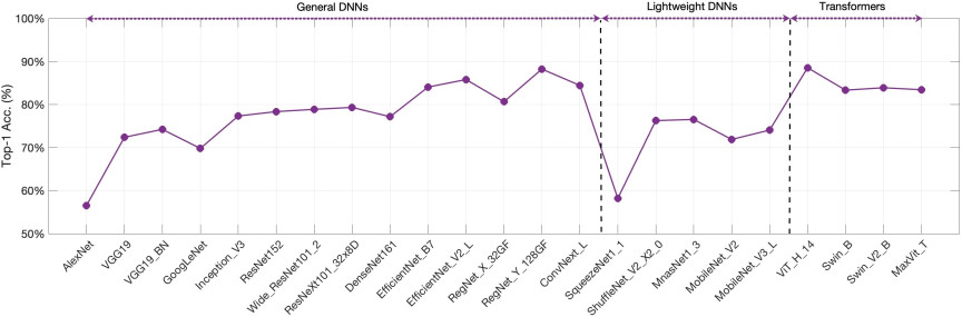
Fig. 1. Top-1 accuracy of typical DNNs.
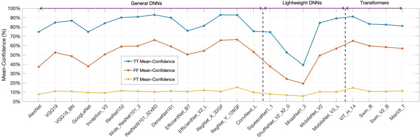
Fig. 2. Mean value of confidence for TT, FF, and FT.
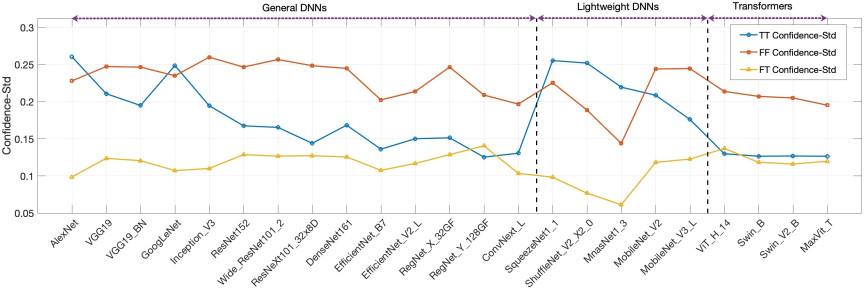
Fig. 3. Standard deviation (Std) of mean confidence for TT, FF, and FT.
To further investigate architecture-dependent confidence behavior at the strongest performance level of each model family, the top-performing network in terms of Top-1 accuracy is selected as the representative model for each architecture. These representative networks are compared from three complementary perspectives, namely classification accuracy, mean confidence of TT/FF/FT predictions, and the corresponding confidence standard deviations.
Representative models of general DNNs, lightweight DNNs, and Transformers all achieve reasonably competitive Top-1 accuracy, as is shown in Fig. 1. However, these accuracy levels do not correspond to a consistent cross-architecture confidence pattern, as illustrated in Fig. 2. In particular, prediction confidence exhibits substantially greater variation across architectures than Top-1 accuracy, suggesting that it captures an additional architecture-sensitive property.
A first observation concerns TT-prediction confidence. In general, stronger CNN and Transformer architectures tend to exhibit higher TT-confidence, indicating that high-performance models often express stronger certainty in correctly classified samples. This trend is observed in several representative high-capacity architectures, suggesting that improved feature representation and stronger global or hierarchical modeling can support both classification correctness and confidence expression. However, this tendency should not be interpreted as a universal rule. For example, EfficientNet_B4 and EfficientNetV2_M provide clear counterexamples, where improved Top-1 accuracy is accompanied by a marked decrease in TT-confidence.
The Transformer family exhibits a confidence signature that, while sharing the high TT-confidence characteristic of strong general DNNs, is further distinguished by a more concentrated and stable distribution of confidence across samples. ViT_H_14, Swin_B, Swin_V2_B, and MaxViT_T maintain TT-confidence values of 91.05%, 83.11%, 82.36%, and 80.97%, respectively, which are all consistently high relative to their accuracy levels. More importantly, as shown in Fig. 3, their TT-confidence standard deviations are all less than 0.1300, which are noticeably lower than those of many CNN representatives. A plausible explanation is that self-attention-based global interaction enables a more coordinated semantic representation, so that the evidence supporting the correct class is distributed more consistently across input samples.
By contrast, lightweight DNNs exhibit much greater variability in TT-confidence than general DNNs and Transformers, despite relatively comparable Top-1 accuracy. This suggests that confidence behavior is more fragile under efficiency-oriented design constraints. Some lightweight models can preserve Top-1 correctness, but their confidence outputs become substantially softer, indicating that architecture compression may retain sufficient discriminative power for correct ranking while weakening the sharpness of the predicted-class probability.
Another cross-architecture phenomenon is that model strengthening often increases confidence in both correct and incorrect predictions. In several depth- or scale-expanded architectures, such as VGG, ResNet, RegNet, ViT, and Swin, higher TT-confidence is accompanied by higher FF-confidence, suggesting that stronger representations may sharpen the output distribution for both correct predictions and certain misclassifications. However, this pattern is not universal; VGG-BN improves the confidence profile by increasing TT-confidence while reducing FF-confidence, whereas EfficientNet and some lightweight models improve or preserve accuracy with softened confidence outputs. These differences indicate that confidence behavior is shaped not only by model capacity, but also by normalization, regularization, scaling strategy, and lightweight design constraints. Therefore, confidence-aware model design and deployment should not only produce confident correct predictions, but also avoid excessive confidence in incorrect predictions and maintain clear correct–incorrect confidence separation.
The confidence standard deviations in Fig. 3 provide further insight into stability. Among the representative lightweight DNNs, SqueezeNet1_1, ShuffleNet_V2_X2_0, and MnasNet1_3 exhibit TT-confidence standard deviations of 0.2556, 0.2522, and 0.2197, respectively, which are all substantially higher than those of ViT_H_14, Swin_B, and MaxViT_T. Even MobileNet_V3_L, which performs relatively well in mean confidence, still has a TT-confidence standard deviation of 0.1762, higher than the Transformer representatives. This demonstrates that confidence stability is itself architecture-dependent. General high-performing CNNs and Transformers not only achieve stronger confidence on average, but also distribute confidence more consistently across samples, whereas lightweight architectures tend to exhibit larger sample-to-sample dispersion. From the viewpoint of deployment, this means that some models may appear satisfactory in terms of mean confidence, yet still behave less reliably because their confidence expression is unstable.
3.5. Discussion
General-CNNs, Lightweight-CNNs, and Transformers differ not only in classification correctness, but also in how certainty is formed, expressed, and distributed. In particular, lightweight designs reveal that confidence-related reliability may degrade well before a substantial drop in Top-1 accuracy becomes visible, whereas Transformers show an advantage in stable certainty expression. These findings imply that reliability-oriented model assessment should explicitly incorporate confidence level, confidence separation, and confidence stability, rather than relying on Top-1 accuracy alone. They also suggest that future lightweight architecture design should treat confidence preservation as an explicit target.
4. Calibration for Prediction Confidence of DNNs
Confidence calibration in the context of DL refers to the alignment between the predicted confidence scores and the actual probability of the model’s predictions. The goal of confidence calibration is to ensure that the confidence scores output by the model are representative of the true probabilities of the events they predict. However, despite not exhibiting overfitting in terms of 0/1 error, contemporary DNNs exhibit suboptimal calibration owing to their extensive capacity, and the negative log-likelihood 44,45. An overconfident incorrect prediction may lead to inappropriate decisions, whereas a well-calibrated confidence score can provide a more reliable indication of prediction uncertainty. Therefore, confidence calibration is an important step toward improving the interpretability and reliability of DNN-based systems.
This section reviews typical calibration methods for DNNs from three perspectives: ensemble-based methods, scaling-based methods, and architecture-level methods.
4.1. Ensembling Mechanisms
Ensemble method refers to the strategy utilizing a set of models to generate aggregated predictions through a voting mechanism. Dietterich 46 provides an analytical explanation of why ensemble methods generally surpass the performance of any single classifier, examining this phenomenon from three distinct perspectives: statistical, computational, and representational.
Lakshminarayanan et al. 47 introduced deep ensembles for the estimation of predictive uncertainty. This approach achieves equally effective or ever superior performance in calibrating uncertainty estimates to that of approximate Bayesian NNs.
Subsequently, in terms of the fully convolutional neural networks (FCNs) applied to medical image segmentation, Mehrtash et al. 48 proposed an innovative approach to enhance the confidence calibration of FCNs through model ensembling. Initially, their research methodically examines the performance and uncertainty estimation capabilities of FCNs, employing both cross-entropy loss and dice loss for evaluation. The findings indicate that although dice loss tends to yield superior segmentation outcomes, it falls short in terms of calibration quality when compared to cross-entropy loss. Building on this insight, the team formulated an ensemble technique that leverages the advantages of dice loss. This method not only improves uncertainty estimation but also enhances the overall quality of segmentation. Let \(M\) represent the quantity of FCN models in the ensemble, \({p_E}\) denote the average probability of the ensembles, the proposed calibration methods with ensembling is expressed as Eq. (6).
The research demonstrates the efficiency of ensembling calibration; it is evidenced that when the ensemble size is greater than or equal to five (\(M \geq 5\)), the confidence calibration is significantly enhanced. Additionally, the segmentation outcomes show marked improvements in terms of the dice coefficient and the Hausdorff distance metrics. Furthermore, the ensemble strategy exhibits superior performance over Monte Carlo dropout methods in the estimation of uncertainty for DL-based image segmenters.
4.2. Scaling Approaches
Scaling for DNN calibration refers to the technique of modifying the scale of the data, typically the output logits of the network, aiming to align the prediction probabilities of the networks with the actual accuracy of the predictions.
Platt scaling derived from the sigmoid function is a well known scaling method originally associated with support vector machines (SVM) 49. Generally, SVM does not inherently output probabilities. Platt scaling is proposed to transform the outputs into a probability distribution over classes. In addition to SVM, Platt scaling is also adaptable to two-classification DNNs. The mathematical expression for Platt scaling is defined as follows:
In the realm of DL with multi-classification tasks, being the extensions of Platt scaling, matrix scaling and vector scaling for multi-class tasks are then developed.
Subsequently, Guo et al. 50 proposed the temperature scaling method to calibrate the prediction confidence of DNNs. The method is denoted as a single parameter variant of Platt scaling by the proposal. The algorithm employs a single scalar parameter \(T\) that modifies the softmax function, i.e., it being applied to the logits of neural networks to calibrate the confidence scores for predictions. In detail, the temperature scaling function is expressed as Eq. (10).
The research in 50 shows that temperature scaling achieves best performance compared to histogram binning 51, isotonic 52, BBQ 53, vector scaling, matrix scaling on computer vision tasks and being comparable to these methods for NLP tasks. Utilizing the post-processing temperature scaling for confidence calibration, Carneiro et al. 54 also developed a new Bayesian DL method based on calibration and uncertainty. And experiments conducted on five-class polyp classification show the efficiency of the proposal holding the state-of-the-art results for confidence calibration and classification accuracy.
Effective confidence calibration helps in enhancing the reliability and interpretability of DNNs, making them more suitable for practical applications where decision-making is based on the model’s predictions.
Focusing on the segmentation for medical images, Mehrtash et al. proposed a model-ensembling method to calibrate the confidence of CNNs. First, they systematically explored the segmentation performance and uncertainty estimation of FCNs utilizing the cross-entropy loss and dice loss, concluding that dice loss generally achieves superior segmentation performance with insuperior calibration compared to cross-entropy. Then, taking the dice loss method, they developed an ensemble method for improving the uncertainty estimation while obtaining higher segmentation quality. In another work, Karimi and Gholipour also indicate that multitask learning significantly improves the confidence calibration of CNN-based segmentation models for medical image 55.
4.3. Architecture-Level Methods
In addition to directly calibrating the confidence levels in DNNs, research also focuses on identifying trustworthy DNN architectures that inherently enhance model trustworthiness.
The confidence level of predictions made by DNNs is intricately linked to the network’s ability to extract, process, distinguish, and utilize the features from the input data. The quality of the feature extraction components, i.e., typically the convolution filters in DNNs, determines the confidence level of the network. However, traditional metrics for prediction accuracy fall short in adequately capturing this aspect. They do not fully reflect the nuanced capabilities of a DNN to process and interpret the complex patterns within the data that are critical for generating reliable predictions. This highlights the need for more sophisticated measures that can assess the quality of feature extraction and its impact on the confidence and trustworthiness of DNN predictions.
In light of this perspective, the generalized feature-based confidence metric (GFBC) is introduced 56. This innovative metric conducts a layer-wise analysis of feature vectors to assess their quality. By evaluating the integrity and discriminative power of these feature vectors, the metric provides a sophisticated measure of the network’s confidence level. For models exhibiting an accuracy variance of no greater than 0.5%, the GFBC metric demonstrates the ability to discriminate among these models based on prediction confidence, with a differentiation range approximately from 1% to 8%. This metric effectively quantifies the subtle distinctions in confidence levels, even among models whose performance metrics are closely aligned, thereby providing a more nuanced understanding of model reliability based on the feature quality of DNNs.
Kumar et al. 45 introduce a strategy that incorporates confidence calibration concurrently with the reduction of classification error during the network training phase. The method leverages the capabilities of reproducing kernel Hilbert space functions, invoked by a universal kernel, to articulate calibration error in the form of an integral probability metric. This metric is termed the maximum mean calibration error, a concept formulated by the authors to facilitate a practical and efficient calibration measure within the training phase of neural networks.
Additionally, confidence assessment issues may stem from unsafe or corner inputs that substantially differ from the training samples, potentially undermining the model’s confidence certainty. In response to this situation, Rossolini et al. 57 propose a lightweight monitoring architecture involving four coverage analysis methods, i.e., single-range coverage, multi-range coverage, \(k\)-nearest neighbors coverage, and neuron rank coverage, to improve the confidence level for unsafe inputs.
4.4. Summary
In summary, these calibration methods improve the reliability of DNN confidence scores at different levels. Calibration method improves the correspondence between confidence scores and empirical correctness, whereas the architecture-dependent confidence patterns observed in this study reveal how network designs intrinsically shape prediction behavior. Together, these perspectives provide a more comprehensive basis for evaluating, selecting, and deploying reliable DNN models.
5. Conclusion
This study presents a unified empirical analysis of prediction-confidence behavior across representative DNN architectures, including General-CNNs, Lightweight-CNNs, and Transformer-based models. The results show that prediction confidence is an essential and architecture-sensitive dimension of DNN behavior that cannot be fully captured by Top-1 accuracy alone. The analysis reveals clear architecture-dependent confidence patterns. In General-CNNs, scaling typically improves Top-1 accuracy, TT-confidence, and confidence concentration, although FF-confidence may also increase. Lightweight-CNNs show the strongest heterogeneity; some preserve confidence capability well, whereas others maintain competitive accuracy while suffering substantial degradation in confidence sharpness and separation. Transformer-based models generally achieve both high TT-confidence and more concentrated confidence distributions, indicating more stable certainty expression across samples. In addition, representative calibration methods are reviewed to situate the empirical findings within the broader context of reliable DNNs. Overall, these findings suggest that confidence level, confidence separation, and confidence stability should all be incorporated into reliability-oriented evaluation of DNNs. By revealing how architectural design shapes prediction-confidence behavior, this study provides guidance for confidence-aware architecture analysis, model design, model optimization, and reliable deployment.
Acknowledgments
This research was partially funded by the Henan Province Key Technologies Research Development Project (Grants Nos.252102211106, 252102320281), the Henan Province Key Research and Development Project (Grants No.241111312000), the Henan Province Key International Science and Technology Cooperation Project (Grants No.251111520400), and the Key R&D Project of Henan Province (Grants No.251111220900).
- [1] L. Alzubaidi, J. Zhang, A. J. Humaidi, A. Al-Dujaili, Y. Duan, O. Al-Shamma, J. Santamaría, M. A. Fadhel, M. Al-Amidie, and L. Farhan, “Review of deep learning: Concepts, CNN architectures, challenges, applications, future directions,” J. of Big Data, Vol.8, Article No.53, 2021. https://doi.org/10.1186/s40537-021-00444-8
- [2] J. Ren, H. Li, A. Wang, K. Saho, and L. Meng, “Radar-based gait analysis by transformer-liked network for dementia diagnosis,” Biomedical Signal Processing and Control, Vol.91, Article No.105986, 2024. https://doi.org/10.1016/j.bspc.2024.105986
- [3] B. Lyu, H. Li, A. Tanaka, and L. Meng, “The early Japanese books reorganization by combining image processing and deep learning,” CAAI Trans. on Intelligence Technology, Vol.7, Issue 4, pp. 627-643, 2022. https://doi.org/10.1049/cit2.12104
- [4] H. Li and L. Meng, “Hardware-aware approach to deep neural network optimization,” Neurocomputing, Vol.559, Article No.126808, 2023. https://doi.org/10.1016/j.neucom.2023.126808
- [5] H. Li, X. Yue, and L. Meng, “Enhanced Mechanisms of Pooling and Channel Attention for Deep Learning Feature Maps,” PeerJ Computer Science, Vol.8, Article No.e1161, 2022. https://doi.org/10.7717/peerj-cs.1161
- [6] H. Li, Z. Wang, X. Yue, W. Wang, H. Tomiyama, and L. Meng, “An architecture-level analysis on deep learning models for low-impact computations,” Artificial Intelligence Review, Vol.56, pp. 1971-2010, 2023. https://doi.org/10.1007/s10462-022-10221-5
- [7] T. Su, Y. Zhang, X. Liang, and N. Ma, “Trajectory Planning Method for Fracture Reduction of Parallel Robots Based on DMP and APF,” IEEE Trans. on Automation Science and Engineering, Vol.23, pp. 4130-4141, 2026. https://doi.org/10.1109/TASE.2026.3653476
- [8] X. Liang, Y. Yan, W. Wang, T. Su, G. He, G. Li, and Z.-G. Hou, “Adaptive Human-Robot Interaction Torque Estimation With High Accuracy and Strong Tracking Ability for a Lower Limb Rehabilitation Robot,” IEEE/ASME Trans. on Mechatronics, Vol.29, Issue 6, pp. 4814-4825, 2024. https://doi.org/10.1109/TMECH.2024.3394491
- [9] S. Liu and W. Deng, “Very deep convolutional neural network based image classification using small training sample size,” 2015 3rd IAPR Asian Conf. on Pattern Recognition (ACPR), pp. 730-734, 2015. https://doi.org/10.1109/ACPR.2015.7486599
- [10] C. Szegedy, W. Liu, Y. Jia, P. Sermanet, S. Reed, D. Anguelov, D. Erhan, V. Vanhoucke, and A. Rabinovich, “Going deeper with convolutions,” 2015 IEEE Conf. on Computer Vision and Pattern Recognition (CVPR), 2015. https://doi.org/10.1109/CVPR.2015.7298594
- [11] S. Ioffe and C. Szegedy, “Batch Normalization: Accelerating Deep Network Training by Reducing Internal Covariate Shift,” The 32nd Int. Conf. on Machine Learning (ICML), Vol.37, pp. 448-456, 2015.
- [12] C. Szegedy, V. Vanhoucke, S. Ioffe, J. Shlens, and Z. Wojna, “Rethinking the Inception Architecture for Computer Vision,” 2016 IEEE Conf. on Computer Vision and Pattern Recognition (CVPR), pp. 2818-2826, 2016. https://doi.org/10.1109/CVPR.2016.308
- [13] K. He, X. Zhang, S. Ren, and J. Sun, “Deep Residual Learning for Image Recognition,” 2016 IEEE Conf. on Computer Vision and Pattern Recognition (CVPR), pp. 770-778, 2016. https://doi.org/10.1109/CVPR.2016.90
- [14] G. Huang, Z. Liu, L. Van Der Maaten, and K. Q. Weinberger, “Densely Connected Convolutional Networks,” 2017 IEEE Conf. on Computer Vision and Pattern Recognition (CVPR), pp. 2261-2269, 2017. https://doi.org/10.1109/CVPR.2017.243
- [15] M. Tan and Q. V. Le, “EfficientNet: Rethinking Model Scaling for Convolutional Neural Networks,” Proc. of the 36th Int. Conf. on Machine Learning, Vol.97, pp. 6105-6114, 2019.
- [16] M. Tan and Q. V. Le, “EfficientNetV2: Smaller Models and Faster Training,” Proc. of the 38th Int. Conf. on Machine Learning, Vol.139, pp. 10096-10106, 2021.
- [17] J. Xu, Y. Pan, X. Pan, S. Hoi, Z. Yi, and Z. Xu, “RegNet: Self-Regulated Network for Image Classification,” IEEE Trans. on Neural Networks and Learning Systems, Vol.34, Issue 11, pp. 9562-9567, 2023. https://doi.org/10.1109/TNNLS.2022.3158966
- [18] Z. Liu, H. Mao, C.-Y. Wu, C. Feichtenhofer, T. Darrell, and S. Xie, “A ConvNet for the 2020s,” 2022 IEEE/CVF Conf. on Computer Vision and Pattern Recognition (CVPR), pp. 11966-11976, 2022. https://doi.org/10.1109/CVPR52688.2022.01167
- [19] F. N. Iandola, S. Han, M. W. Moskewicz, K. Ashraf, W. J. Dally, and K. Keutzer, “Squeezenet: Alexnet-level accuracy with 50× fewer parameters and <0.5MB model size,” arXiv:1602.07360, 2016. https://doi.org/10.48550/arXiv.1602.07360
- [20] A. G. Howard, M. Zhu, B. Chen, D. Kalenichenko, W. Wang, T. Weyand, M. Andreetto, and H. Adam, “MobileNets: Efficient Convolutional Neural Networks for Mobile Vision Applications,” arXiv:1704.04861, 2017. https://doi.org/10.48550/arXiv.1704.04861
- [21] M. Sandler, A. Howard, M. Zhu, A. Zhmoginov, and L.-C. Chen, “MobileNetV2: Inverted Residuals and Linear Bottlenecks,” 2018 IEEE/CVF Conf. on Computer Vision and Pattern Recognition, pp. 4510-4520, 2018. https://doi.org/10.1109/CVPR.2018.00474
- [22] X. Zhang, X. Zhou, M. Lin, and J. Sun, “ShuffleNet: An Extremely Efficient Convolutional Neural Network for Mobile Devices,” 2018 IEEE Conf. on Computer Vision and Pattern Recognition (CVPR), pp. 6848-6856, 2018. https://doi.org/10.1109/CVPR.2018.00716
- [23] N. Ma et al., “ShuffleNet V2: Practical Guidelines for Efficient CNN Architecture Design,” The 15th European Conf. on Computer Vision (ECCV), pp. 122-138, 2018. https://doi.org/10.1007/978-3-030-01264-9_8
- [24] M. Tan, B. Chen, R. Pang, V. Vasudevan, M. Sandler, A. Howard, and Q. V. Le, “MnasNet: Platform-Aware Neural Architecture Search for Mobile,” 2019 IEEE/CVF Conf. on Computer Vision and Pattern Recognition (CVPR), pp. 2815-2823, 2019. https://doi.org/10.1109/CVPR.2019.00293
- [25] Z. Liu, Y. Lin, Y. Cao, H. Hu, Y. Wei, Z. Zhang, S. Lin, and B. Guo, “Swin Transformer: Hierarchical Vision Transformer using Shifted Windows,” 2021 IEEE/CVF Int. Conf. on Computer Vision (ICCV), pp. 9992-10002, 2021. https://doi.org/10.1109/ICCV48922.2021.00986
- [26] A. Dosovitskiy, L. Beyer, A. Kolesnikov, D. Weissenborn, X. Zhai, T. Unterthiner, M. Dehghani, M. Minderer, G. Heigold, S. Gelly, J. Uszkoreit, and N. Houlsby, “An Image is Worth 16×16 Words: Transformers for Image Recognition at Scale,” Int. Conf. on Learning Representations, 2021.
- [27] Z. Tu, H. Talebi, H. Zhang, F. Yang, P. Milanfar, A. Bovik, and Y. Li, “MaxViT: Multi-axis Vision Transformer,” The 17th European Conf. on Computer Vision (ECCV 2022), pp. 459-479, 2022. https://doi.org/10.1007/978-3-031-20053-3_27
- [28] X. Xu, M. Xie, P. Miao, W. Qu, W. Xiao, H. Zhang, X. Liu, and T.-T. Wong, “Perceptual-Aware Sketch Simplification Based on Integrated VGG Layers,” IEEE Trans. on Visualization and Computer Graphics, Vol.27, Issue 1, pp. 178-189, 2021. https://doi.org/10.1109/TVCG.2019.2930512
- [29] H. Zhou, W. Chen, L. Cheng, D. Williams, C. W. De Silva, and M. Xia, “Reliable and Intelligent Fault Diagnosis With Evidential VGG Neural Networks,” IEEE Trans. on Instrumentation and Measurement, Vol.72, 2023. https://doi.org/10.1109/TIM.2023.3250308
- [30] S.-H. Wang, S. L. Fernandes, Z. Zhu, and Y.-D. Zhang, “AVNC: Attention-Based VGG-Style Network for COVID-19 Diagnosis by CBAM,” IEEE Sensors J., Vol.22, Issue 18, pp. 17431-17438, 2022. https://doi.org/10.1109/JSEN.2021.3062442
- [31] A. Sepas-Moghaddam, M. A. Haque, P. L. Correia, K. Nasrollahi, T. B. Moeslund, and F. Pereira, “A Double-Deep Spatio-Angular Learning Framework for Light Field-Based Face Recognition,” IEEE Trans. on Circuits and Systems for Video Technology, Vol.30, Issue 12, pp. 4496-4512, 2020. https://doi.org/10.1109/TCSVT.2019.2916669
- [32] X. Ren, H. Mosavat-Jahromi, L. Cai, and D. Kidston, “Spatio-Temporal Spectrum Load Prediction Using Convolutional Neural Network and ResNet,” IEEE Trans. on Cognitive Communications and Networking, Vol.8, Issue 2, pp. 502-513, 2022. https://doi.org/10.1109/TCCN.2021.3139030
- [33] P. Guo, H. Dai, Q. Yang, Q. Huang, and H. Yao, “An Improved Magnetic Tracking Approach Based on ResNet-LM Fusion Algorithm,” IEEE Trans. on Instrumentation and Measurement, Vol.71, 2022. https://doi.org/10.1109/TIM.2022.3216597
- [34] Z. Zhu, W. Zhai, H. Liu, J. Geng, M. Zhou, C. Ji, and G. Jia, “Juggler-ResNet: A Flexible and High-Speed ResNet Optimization Method for Intrusion Detection System in Software-Defined Industrial Networks,” IEEE Trans. on Industrial Informatics, Vol.18, Issue 6, pp. 4224-4233, 2022. https://doi.org/10.1109/TII.2021.3121783
- [35] D. O’Neill, B. Xue, and M. Zhang, “Evolutionary Neural Architecture Search for High-Dimensional Skip-Connection Structures on DenseNet Style Networks,” IEEE Trans. on Evolutionary Computation, Vol.25, Issue 6, pp. 1118-1132, 2021. https://doi.org/10.1109/TEVC.2021.3083315
- [36] F. Yuwei, L. Liejuan, H. Weihua, H. Guobin, H. Peijun, Z. Zhiyu, C. Chi, and W. Chuang, “Partial Discharge Pattern Recognition Method Based on Transfer Learning and DenseNet Model,” IEEE Trans. on Dielectrics and Electrical Insulation, Vol.30, Issue 3, pp. 1240-1246, 2023. https://doi.org/10.1109/TDEI.2023.3239032
- [37] L. Huang and C.-M. Pun, “Audio Replay Spoof Attack Detection by Joint Segment-Based Linear Filter Bank Feature Extraction and Attention-Enhanced DenseNet-BiLSTM Network,” IEEE/ACM Trans. on Audio, Speech, and Language Processing, Vol.28, pp. 1813-1825, 2020. https://doi.org/10.1109/TASLP.2020.2998870
- [38] N. K. Yadav, S. K. Singh, and S. R. Dubey, “MobileAR-GAN: MobileNet-Based Efficient Attentive Recurrent Generative Adversarial Network for Infrared-to-Visual Transformations,” IEEE Trans. on Instrumentation and Measurement, Vol.71, 2022. https://doi.org/10.1109/TIM.2022.3166202
- [39] J. Yang, Y. Wang, H. Zhao, and G. Gui, “MobileNet and Knowledge Distillation-Based Automatic Scenario Recognition Method in Vehicle-to-Vehicle Systems,” IEEE Trans. on Vehicular Technology, Vol.71, Issue 10, pp. 11006-11016, 2022. https://doi.org/10.1109/TVT.2022.3184994
- [40] T. Addabbo, A. Fort, M. Mugnaini, V. Vignoli, M. Intravaia, M. Tani, M. Bianchini, F. Scarselli, and B. T. Corradini, “Smart Gravimetric System for Enhanced Security of Accesses to Public Places Embedding a MobileNet Neural Network Classifier,” IEEE Trans. on Instrumentation and Measurement, Vol.71, 2022. https://doi.org/10.1109/TIM.2022.3162270
- [41] A. Lin, B. Chen, J. Xu, Z. Zhang, G. Lu, and D. Zhang, “DS-TransUNet: Dual Swin Transformer U-Net for Medical Image Segmentation,” IEEE Trans. on Instrumentation and Measurement, Vol.71, 2022. https://doi.org/10.1109/TIM.2022.3178991
- [42] X. Meng, Y. Yang, L. Wang, T. Wang, R. Li, and C. Zhang, “Class-Guided Swin Transformer for Semantic Segmentation of Remote Sensing Imagery,” IEEE Geoscience and Remote Sensing Letters, Vol.19, 2022. https://doi.org/10.1109/LGRS.2022.3215200
- [43] F. Sun, W. Zhou, L. Ye, and L. Yu, “Hierarchical Decoding Network Based on Swin Transformer for Detecting Salient Objects in RGB-T Images,” IEEE Signal Processing Letters, Vol.29, pp. 1714-1718, 2022. https://doi.org/10.1109/LSP.2022.3194843
- [44] C. Zhang, S. Bengio, M. Hardt, B. Recht, and O. Vinyals, “Understanding deep learning (still) requires rethinking generalization,” Commun. ACM, Vol.64, Issue 3, pp. 107-115, 2021. https://doi.org/10.1145/3446776
- [45] A. Kumar, S. Sarawagi, and U. Jain, “Trainable Calibration Measures for Neural Networks from Kernel Mean Embeddings,” Proc. of the 35th Int. Conf. on Machine Learning, Vol.80, pp. 2805-2814, 2018.
- [46] T. G. Dietterich, “Ensemble Methods in Machine Learning,” Int. Workshop on Multiple Classifier Systems (MCS 2000), 2000. https://doi.org/10.1007/3-540-45014-9_1
- [47] B. Lakshminarayanan, A. Pritzel, and C. Blundell, “Simple and Scalable Predictive Uncertainty Estimation using Deep Ensembles,” Proc. of the 31st Int. Conf. on Neural Information Processing Systems, pp. 6405-6416, 2017.
- [48] A. Mehrtash, W. M. Wells, C. M. Tempany, P. Abolmaesumi, and T. Kapur, “Confidence Calibration and Predictive Uncertainty Estimation for Deep Medical Image Segmentation,” IEEE Trans. on Medical Imaging, Vol.39, Issue 12, pp. 3868-3878, 2020. https://doi.org/10.1109/TMI.2020.3006437
- [49] J. C. Platt, “Probabilistic Outputs for Support Vector Machines and Comparisons to Regularized Likelihood Methods,” Advances in Large Margin Classifiers, Vol.10, No.3, pp. 61-74, 1999.
- [50] C. Guo, G. Pleiss, Y. Sun, and K. Q. Weinberger, “On Calibration of Modern Neural Networks,” Proc. of the 34th Int. Conf. on Machine Learning, Vol.70, pp. 1321-1330, 2017.
- [51] B. Zadrozny and C. Elkan, “Obtaining calibrated probability estimates from decision trees and naive Bayesian classifiers,” Proc. of the 18th Int. Conf. on Machine Learning, pp. 609-616, 2001.
- [52] B. Zadrozny and C. Elkan, “Transforming classifier scores into accurate multiclass probability estimates,” Proc. of the 8th ACM SIGKDD Int. Conf. on Knowledge Discovery and Data Mining, pp. 694-699, 2002. https://doi.org/10.1145/775047.775151
- [53] M. P. Naeini, G. Cooper, and M. Hauskrecht, “Obtaining Well Calibrated Probabilities Using Bayesian Binning,” Proc. of the 29th AAAI Conf. on Artificial Intelligence, pp. 2901-2907, 2015. https://doi.org/10.1609/aaai.v29i1.9602
- [54] G. Carneiro, L. Z. C. T. Pu, R. Singh, and A. Burt, “Deep learning uncertainty and confidence calibration for the five-class polyp classification from colonoscopy,” Medical Image Analysis, Vol.62, Article No.101653, 2020. https://doi.org/10.1016/j.media.2020.101653
- [55] D. Karimi and A. Gholipour, “Improving Calibration and Out-of-Distribution Detection in Deep Models for Medical Image Segmentation,” IEEE Trans. on Artificial Intelligence, Vol.4, Issue 2, pp. 383-397, 2023. https://doi.org/10.1109/TAI.2022.3159510
- [56] M. A. Haghpanah, M. T. Masouleh, and A. Kalhor, “Determining the trustworthiness of DNNs in classification tasks using generalized feature-based confidence metric,” Pattern Recognition, Vol.142, Article No.109683, 2023. https://doi.org/10.1016/j.patcog.2023.109683
- [57] G. Rossolini, A. Biondi, and G. Buttazzo, “Increasing the Confidence of Deep Neural Networks by Coverage Analysis,” IEEE Trans. on Software Engineering, Vol.49, Issue 2, pp. 802-815, 2023. https://doi.org/10.1109/TSE.2022.3163682
This article is published under a Creative Commons Attribution-NoDerivatives 4.0 Internationa License.