
Research Paper:
Semantic-Topological Cognitive Maps for Assistive Indoor Navigation of a Robot Partner
Anhar Risnumawan*,**
 , Achmad Fahrul Aji*,***
, Raditya Artha Rochmanto*,***
, Teuku Zikri Fatahillah*
, and Naoyuki Kubota*,†
*Department of Mechanical Systems Engineering, Graduate School of Systems Design, Tokyo Metropolitan University
6-6 Asahigaoka, Hino, Tokyo 191-0065, Japan
†Corresponding author
**Mechatronics Engineering Division, Politeknik Elektronika Negeri Surabaya
Jalan Raya ITS, Surabaya 60111, Indonesia
***Department of Electrical Engineering, Politeknik Negeri Semarang
Jl. Prof. H. Soedarto SH, Tembalang, Semarang 50275, Indonesia

Assistive indoor mobile robots are increasingly expected to connect natural-language requests about familiar places and objects with the metric maps used for localization and motion planning. Metric simultaneous localization and mapping (SLAM) supports reliable geometry and collision avoidance, whereas many open-vocabulary scene-graph systems remain separated from the navigation stacks used on deployed robots. This paper presents a semantic-topological cognitive map (STCM) that bridges these representations for assistive navigation. The system derives place nodes from a LiDAR–inertial pose stream through a dual growing neural gas backend and consolidates object instances over time. GroundingDINO and MobileSAM provide open-vocabulary semantic grounding in the map frame through LiDAR–image association and temporal score fusion. A tool-mediated large language model interface maps user commands to explicit STCM nodes, while graph search and ROS 2 Navigation2 (Nav2) remain responsible for path computation and execution. Evaluation with recorded robot sessions, an outdoor distribution-shift probe, and a public indoor-scene benchmark indicates that the STCM backend improves object-graph construction and that the language interface improves functional-command grounding when requested objects are recoverable by perception. The pipeline is demonstrated on a Ranger Garden Assistant platform with FAST-LIO2 mapping, incremental graph construction during the mapping pass, and waypoint execution from a serialized map artifact.
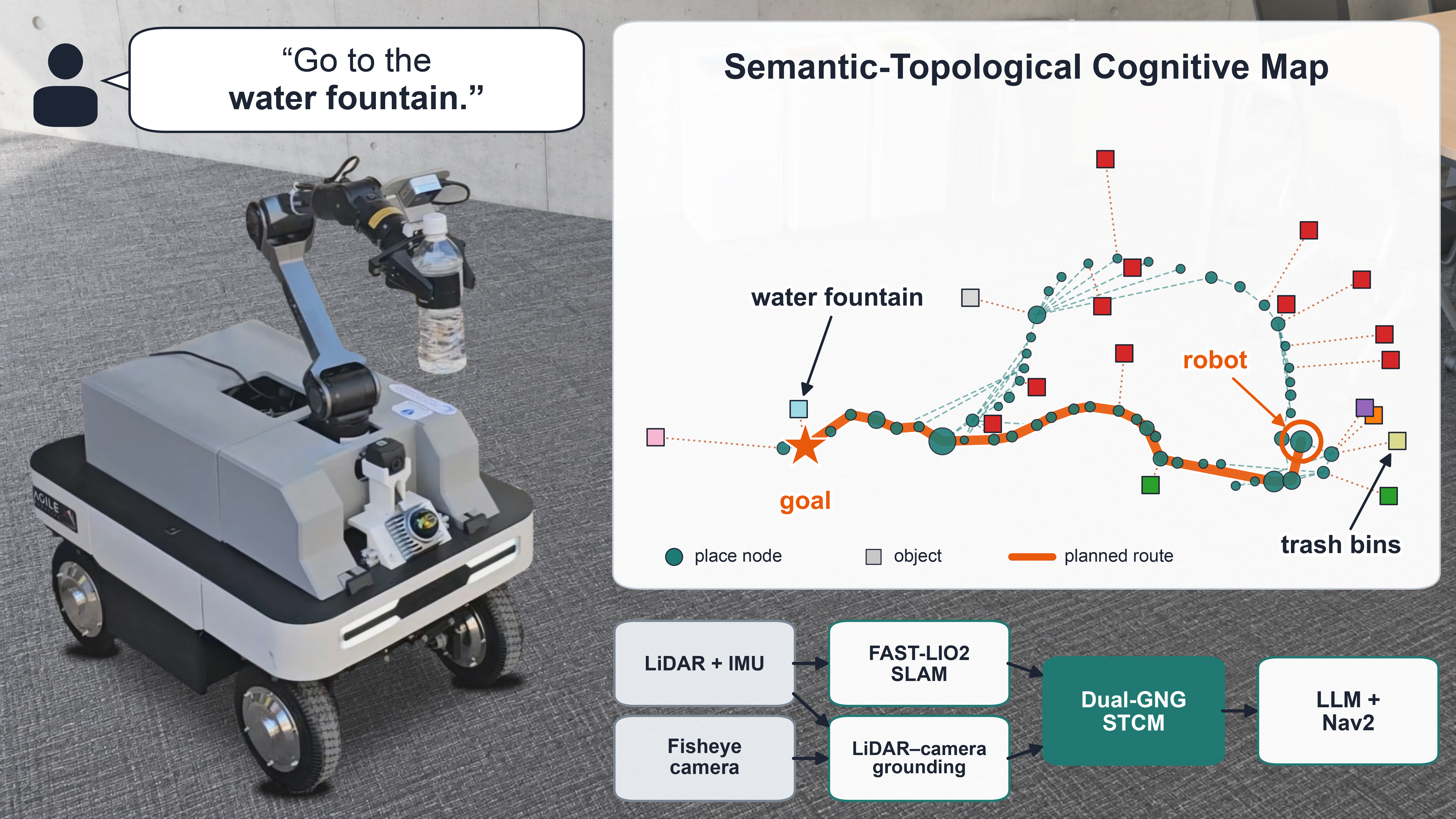
Ranger Garden Assistant platform with semantic topological cognitive map
1. Introduction
Assistive indoor mobile robots are increasingly expected to operate in environments that people describe in terms of places, objects, and everyday tasks. In aging-society homes and care settings, users are unlikely to specify metric coordinates or manually selected waypoints. They are more likely to issue commands such as “go to the kitchen,” “find my medicine,” or “bring it to my bedside.” Such requests assume that the robot can connect symbolic place and object concepts to the geometric world in which it localises and moves. A useful assistive navigation representation must therefore provide a stable, labelled spatial structure that supports repeated reference to familiar places and objects while remaining inspectable by designers, operators, and downstream planning modules. Perceived reliability and understandable robot behaviour are recognized as factors that shape trust in human–robot interaction (HRI) 1, so an assistive robot should expose its spatial knowledge at the level of nodes, labels, and navigation choices rather than hide it inside an opaque end-to-end policy. Fig. 1 illustrates this setting: a robot partner must connect natural-language commands to familiar places and objects through an explicit semantic-topological map.
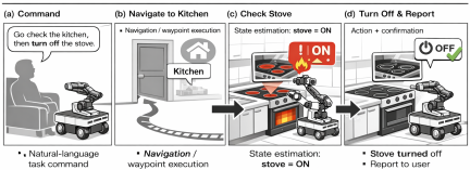
Fig. 1. Illustration of an assistive indoor navigation scenario. A robot partner must understand natural language commands that refer to familiar places (kitchen, bedside) and objects (medicine) rather than coordinates.
This need for an explicit semantic-topological map can be framed through multi-scopic models of intelligent behaviour. Such models describe cognition across micro-, meso-, and macroscopic levels, linking sensing, perception, and cognition 2. For navigation, this view motivates a representation that combines metric sensing for local motion, topological structure for place connectivity, and semantic labels for task-level reasoning.
Building on this multi-scopic view, metric simultaneous localization and mapping (SLAM) provides the geometric layer needed for localization, collision checking, and precise motion planning. It produces a pose stream and a geometric map, but this metric representation alone does not encode the discrete place concepts required for language-grounded navigation. It does not directly represent “kitchen,” “bedside,” “doorway,” or “next to the table.” This limitation motivates place-based abstraction, drawing on cognitive maps, ecological affordances, symbolic grounding, and topological reconstruction 3,4,5,6,7.
Recent mapping and navigation systems address important parts of this problem, but they do not fully close the deployment gap. Hierarchical semantic mapping and 3D scene-graph systems, including Kimera 8, Hydra 9, and S-Graphs+ 10, integrate geometric mapping with structured semantic entities. These systems provide rich representations, but they are often oriented toward object-, room-, or building-level structure and global optimization rather than compact, promptable place nodes for language-conditioned navigation. Open-vocabulary systems such as VLMaps 11, ConceptFusion 12, ConceptGraphs 13, and OneMap 14 make maps queryable with flexible language-like concepts, but their representations are commonly dense feature fields or object-centric graphs. They do not directly provide an incrementally constructed, temporally stabilized, node-addressable place graph that can be serialized and executed through standard navigation stacks.
Language-integrated systems further connect natural-language instructions to spatial plans. NLMap, LM-Nav, and GOAT ground language-driven planning in queryable scene representations, graph search, or instance-aware semantic memory 15,16,17. OpenIN, zero-shot language-conditioned mapping, and MapNav extend this direction toward open-vocabulary, language-conditioned navigation stacks 18,19,20. Learned and explicit topological systems, including neural topological SLAM, ETPNav, and RoboHop, also show the value of graph abstractions for long-horizon planning 21,22,23. Across these lines, however, execution is often custom or simulator-centered, semantics may remain latent, and the output is rarely a compact ROS 2/Nav2-ready place graph that can be inspected, edited, addressed by an LLM, and executed on a real light detection and ranging (LiDAR) robot.
This paper addresses that gap with the semantic-topological cognitive map (STCM), a compact place graph constructed incrementally from a LiDAR-inertial pose stream during an initial mapping traversal and serialized as an inspectable stcm.json artifact containing place nodes, labels, confidence scores, object instances, and connectivity. A metric layer based on FAST-LIO2-style LiDAR–inertial SLAM supplies map-frame localization 24, while a topological layer uses growing neural gas (GNG) to learn revisitable place nodes from the robot trajectory 25, with multi-scale GNG variants providing the broader basis for dynamic distributions 26. A semantic layer grounds open-vocabulary detections from GroundingDINO and the segment anything model (SAM), in its lightweight MobileSAM variant 27,28,29, by associating segmentation masks with projected LiDAR points and transforming the anchors into the SLAM map frame through Robot Operating System 2 (ROS 2) TF. Semantic evidence is fused into node-level score vectors, and the language interface gives a large language model (LLM) the user command and serialized graph so that it returns a graph-grounded goal, such as a target node identifier, rather than an end-to-end navigation policy. This design follows prior work on LLMs as high-level planners with explicit affordances, such as SayCan 30, and evidence that structured graph-form inputs can improve LLM spatial reasoning in path-planning settings 31; graph search and low-level execution remain with the planner and ROS 2 Navigation2 (Nav2) 32.
This work makes four contributions:
-
・
A LiDAR-anchored STCM open-vocabulary grounding pipeline that combines GroundingDINO, MobileSAM, LiDAR–image association, map-frame transformation, and temporal node-level semantic fusion.
-
・
An incremental semantic-topological graph backend using dual GNG, constructed during a mapping traversal: place-level nodes are learned from the LiDAR-inertial trajectory, while instance-level GNG consolidates object observations.
-
・
A tool-mediated language-to-graph interface that grounds commands to explicit STCM nodes instead of delegating navigation control to the language model.
-
・
A real-platform ROS 2/Nav2 deployment path from a serialized semantic-topological graph to waypoint execution on a Ranger Garden Assistant platform.
The scope is intentionally practical. STCM is a middle-layer representation between dense open-vocabulary maps and full 3D dynamic scene graphs: it preserves metric mapping for local control while exposing a serializable place graph constructed during mapping for language grounding. The paper supports an integration claim rather than universal benchmark superiority; richer hierarchy, object–object relations, dynamic scene modelling, and user studies remain future work.
2. Related Work
Place-based navigation has long been motivated by cognitive-map, affordance, and informationally structured space models, which treat navigation as more than metric motion through coordinates 3,4,5,7,6. STCM uses this literature as design motivation, not as a tested model of biological cognition.
In robotics, this view supports graph representations whose nodes correspond to revisitable places, decision points, and task-relevant semantic regions. GNG provides one mechanism for incrementally learning such graphs from streaming observations 25,26. Metric-semantic SLAM and 3D scene-graph systems extend this idea by maintaining semantic structure together with geometric estimation. Structured scene graphs 33,34, Kimera and Kimera-Multi 8,35, Hydra 9, S-Graphs+ 10, and modular semantic-mapping architectures 36 provide increasingly rich object-, room-, building-, and geometry-level representations. Their strength is expressive hierarchical mapping and global consistency; STCM differs by intentionally using a lighter serializable place graph tied to a LiDAR-inertial pose stream, open-vocabulary object evidence, and direct Nav2 waypoint execution.
Foundation-model mapping has broadened semantic navigation beyond closed vocabularies. VLMaps and VLFM use vision–language features for zero-shot semantic navigation and exploration 11,37; ConceptFusion, ConceptGraphs, and OneMap build open-set dense maps or object-centric graph representations for spatial queries and downstream planning 12,13,14; and semantic exploration methods show how semantic predictions can guide active search 38. These systems are closest to STCM in open-vocabulary capability, but their main map products are usually dense feature fields, reconstructed 3D features, or object-centric graphs. STCM instead fuses detections into persistent place-node score vectors anchored through LiDAR–image association in the SLAM map frame.
Language-driven navigation systems connect queryable representations to instruction following. NLMap, LM-Nav, GOAT, OpenIN, zero-shot language-conditioned mapping, MapNav, SORT3D, MSGNav, and LagMemo demonstrate language grounding over semantic maps, topological structures, instance memory, 3D scene graphs, or 3D Gaussian-splatting memories 15,16,17,18,19,20,39,40,41. These works provide stronger benchmark coverage for embodied navigation, dynamic instance memory, or relational 3D reasoning than the present evaluation. STCM is complementary: it constrains the LLM to return graph-referenced goals while graph search and Nav2 retain path computation and motion execution on a recorded real LiDAR platform.
Explicit topological navigation methods further support long-horizon planning with graph abstractions. Neural topological SLAM, ETPNav, and RoboHop demonstrate the value of learned or segment-based topology for navigation and semantic querying 21,22,23. Their semantics may be latent, image-segment based, or benchmark-oriented, whereas STCM uses LiDAR-anchored place nodes, persistent node-level semantic fusion, and a ROS 2/Nav2 execution path.
Recent semantic-navigation surveys similarly identify semantic information as a missing middle layer between low-level metric navigation and high-level task intent 42,43. STCM contributes to this middle layer by keeping the representation compact enough for inspection and graph search while retaining metric anchoring for execution.
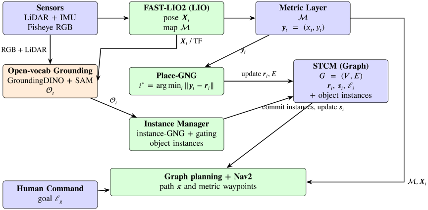
Fig. 2. STCM system pipeline architecture. The pipeline integrates metric SLAM (FAST-LIO2), open-vocabulary grounding (GroundingDINO + SAM), dual-GNG learning (place-GNG for revisitable place nodes and an instance-GNG manager for persistent object instances), and ROS 2 Nav2 execution. Sensor inputs flow through LiDAR-inertial odometry to produce a metric map and pose stream, while open-vocabulary detections are grounded into the map frame and managed as object instances. Place–object associations temporally fuse semantic evidence into node-level score vectors, yielding an STCM graph that supports language-based goal specification, graph planning, and metric waypoint execution.
3. Methodology
3.1. System Architecture and Design Philosophy
The STCM system integrates modern ROS 2 navigation infrastructure with topological learning and semantic labeling for assistive navigation tasks. The architecture maintains a dual representation: a continuous metric map for precise local control and obstacle avoidance, and a discrete topological place graph for task-level planning, semantic grounding, and interpretable communication with users.
Conceptually, STCM is organized across three coupled levels following the multi-scopic framing introduced as motivation. The microscopic level couples real-time metric SLAM with frame-by-frame open-vocabulary detection for short-term sensorimotor feedback such as continuous pose tracking and immediate obstacle reaction. The macroscopic level couples the place graph with a graph-based path planner for long-term deliberative behaviour such as global route planning and persistent place labeling. Between them, the mesoscopic level maintains topological structure learning and localization, integrating bottom-up sensor observations with top-down graph knowledge to support medium-term adaptation: incremental node creation, edge updates, and replanning when environmental change invalidates the current path. This organization lets STCM respond both reactively to immediate obstacles and deliberatively to high-level goals, and is used here as a design heuristic rather than as a claim about a tested cognitive model 2.
The core components operate in a pipeline architecture. Sensor inputs from a 176° field-of-view (FOV) fisheye camera and Livox Mid-360 3D LiDAR are fused with inertial measurements. A LiDAR-inertial odometry (LIO) module based on FAST-LIO2 provides real-time pose estimation \(\boldsymbol{X}_t\) and constructs a metric map \(\mathcal{M}\) via iterative least-squares minimization of LiDAR-inertial residuals 24. The robot’s 2D position in the map frame \(\boldsymbol{y}_t = (x_t, y_t)\) is extracted from the 6-DOF pose and serves as input to the topological learning layer.
The topological layer employs a dual GNG architecture 25,26. A place-level GNG incrementally learns place nodes from the streaming pose observations: at each step the current position \(\boldsymbol{y}_t\) is associated with the nearest existing prototype \(\boldsymbol{r}_i\) through \(i^* = \arg\min_i \|\boldsymbol{y}_t - \boldsymbol{r}_i\|\), and a new place node is created whenever the distance to all existing nodes exceeds the threshold \(D_{\text{new}}\). Edges are added either by local prototype proximity or by observed traversal, encoding navigable connectivity. In parallel, a per-class instance-level GNG operates on detected object positions, clustering multiple instances of the same semantic class—so that three distinct chairs are kept distinct—while suppressing spurious detections through adaptive prototype learning.
Semantic grounding uses open-vocabulary object detection by GroundingDINO, optionally refined by the SAM 27,28. To anchor detections in the map frame, the LiDAR point cloud is projected into the image, and points whose pixel coordinates fall inside a detection mask are taken as the object’s geometric support; the resulting evidence is recorded as \(\mathcal{O}_t = \{(l_i, \boldsymbol{p}_i^{\text{map}}, c_i)\}_i\) with class label \(l_i\), map-frame position \(\boldsymbol{p}_i^{\text{map}}\), and detection confidence \(c_i\). Monocular depth from Depth Anything is held in reserve as an optional fallback when no projected LiDAR point falls inside a mask 44. Place-node semantic score vectors \(\boldsymbol{s}_i\) are updated directly from these per-frame observations, while the instance-level GNG separately clusters the same observations into stable object instances for object-level queries and inspection; the dominant class label \(\ell_i = \arg\max_c s_{i,c}\) becomes the place-node label exposed to the language interface.
The resulting STCM graph \(G = (V, E)\) consists of nodes \(V\) with attributes \(\{\boldsymbol{r}_i, \boldsymbol{s}_i, \ell_i\}\) and edges \(E\) representing traversable connections. Navigation proceeds in two stages: high-level graph planning selects a sequence of place nodes based on semantic goals (e.g., “go to the water fountain”), and low-level execution uses Nav2 to follow metric waypoints corresponding to the selected nodes 32. This architecture enables both symbolic reasoning over place concepts and reactive, collision-free control.
Figure 2 illustrates the complete STCM pipeline architecture, showing the flow from sensor inputs through metric SLAM, semantic grounding, topological learning, and navigation execution.
3.2. Metric Layer: LiDAR-Inertial Odometry and Mapping
The metric layer employs FAST-LIO2, a computationally efficient LiDAR-inertial odometry system that tightly couples 3D LiDAR measurements with inertial data 24. FAST-LIO2 reports competitive or superior localization accuracy at substantially lower computational cost than other state-of-the-art LiDAR-inertial systems across the indoor and outdoor benchmarks evaluated in the original paper 24, providing an accurate metric foundation for STCM’s topological and semantic layers. The system formulates odometry as an iterative extended Kalman filter (iEKF) that estimates the robot state \(\boldsymbol{X}_t = [\boldsymbol{p}_t, \boldsymbol{v}_t, \boldsymbol{q}_t, \boldsymbol{b}_a, \boldsymbol{b}_g]\), where \(\boldsymbol{p}_t\) is position, \(\boldsymbol{v}_t\) is velocity, \(\boldsymbol{q}_t\) is orientation (quaternion), and \(\boldsymbol{b}_a, \boldsymbol{b}_g\) are accelerometer and gyroscope biases. The system maintains an incremental k-d tree (ikd-Tree) representation of the map \(\mathcal{M}\) for efficient nearest-neighbor queries during scan matching.
At each iteration, IMU measurements propagate the state forward via the standard kinematic model. LiDAR points are then registered to the map by solving a point-to-plane iterative closest point (ICP) problem. The measurement residual for point \(j\) in scan \(t\) is defined as in Eq. (1):
The output of FAST-LIO2 is a high-rate pose stream (typically 10–20 Hz in other deployments; in our configuration it is bounded by the 10 Hz Livox scan rate and, under full-system load, was measured at \(7.7\) Hz, Section 5.6) and an odometric point cloud map \(\mathcal{M}\) that is locally consistent within the odometry session; FAST-LIO2 does not by itself provide loop closure or global pose-graph optimization, so global consistency under long revisits is not claimed. For STCM, we extract the planar components \((x_t, y_t)\) of the estimated position \(\boldsymbol{p}_t\) and denote the resulting 2D position stream as \(\boldsymbol{y}_t := [x_t, y_t]^\top\). This stream drives the topological learning module and provides the frame for anchoring semantic detections.
3.3. Topological Layer (Place-GNG) for Place Discovery
GNG is an unsupervised incremental clustering algorithm that adapts its topology and number of nodes online in response to input data 25. We adopt GNG as the topological-learning mechanism in STCM because it offers a compact representation between dense metric maps and sparse landmarks while remaining computationally light, following its use in related online topological mapping work 45. We employ GNG to convert the continuous trajectory \(\{\boldsymbol{y}_t\}\) from SLAM into a discrete place graph suitable for symbolic reasoning and planning. The topological abstraction enables efficient graph-level planning with far fewer nodes than grid cells, making computation tractable without losing essential connectivity information 45. Fig. 3 illustrates the place-GNG mechanism as the robot traverses a corridor, showing node insertion, adaptation, edge creation, and semantic association.
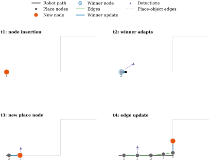
Fig. 3. Place-level GNG illustration. As the robot traverses the corridor, new nodes are inserted when the current pose is farther than \(D_{\text{new}}\) from existing prototypes, and nearby nodes adapt toward revisited poses. Edges may arise from prototype proximity, observed transitions between successive winners, or both. Purple triangles represent object detections, and dashed purple links show the per-frame observation-to-place associations used for semantic fusion.
3.3.1. Node Association and Adaptation
At each time step \(t\), the current robot position \(\boldsymbol{y}_t\) is presented to the GNG network. The algorithm computes distances to all existing nodes as in Eq. (2):
The winner node’s prototype is adapted toward the input using a learning rate \(\epsilon_b\) as in Eq. (4):
3.3.2. Edge Creation and Aging
Connectivity in the place graph is established through two complementary edge-update rules that are both active in STCM configuration, together with a shared aging mechanism. First, following the standard GNG mechanism, when the winner \(i^*\) is determined an edge is created or refreshed between \(i^*\) and the second-nearest node \(i_2\) as in Eq. (6):
3.3.3. Node Insertion
If the robot moves to a region not well represented by existing nodes, a new place node is created. The insertion criterion is given in Eq. (8):
Alternatively, standard GNG uses an error-driven insertion strategy: nodes accumulate error proportional to their distance to inputs, and periodically the node with maximum error spawns a new node between itself and its neighbor with the highest error. For real-time mapping, we favor the distance-threshold criterion for predictable memory usage and computational cost.
The winner–second-nearest rule of Eq. (3) requires at least two prototypes, and the GNG backend cannot represent a single-prototype graph: it defers initialization until two pose samples exist and then seeds exactly two prototypes. The place graph is therefore cold-started by duplicating the first pose \(\boldsymbol{y}_t\), seeding two coincident prototypes at \(\boldsymbol{y}_t\); the winner–second-nearest rule is active from that point onward, and a pose farther than \(D_{\text{new}}\) from its current winner instantiates each subsequent prototype. The second-nearest term \(i_2\) is thus undefined only for the single degenerate transient before the two seeds exist.
3.4. Semantic Grounding Pipeline
The semantic grounding pipeline transforms raw RGB images and LiDAR measurements into labeled 3D object anchors that are fused into the STCM graph. In the STCM configuration, the pipeline consists of six stages: open-vocabulary detection on scene-specific prompt banks, box-prompted instance segmentation, calibrated label rerank via a separate vision–language encoder with an explicit abstention gate, metric grounding through image-projected LiDAR with a voxel-mode pose lift, map-frame observation output, and fusion into place nodes.
3.4.1. Stage 1: Open-Vocabulary Detection
GroundingDINO is a transformer-based detector that conditions on text prompts to detect objects in arbitrary categories without task-specific fine-tuning 27. The model achieves strong zero-shot detection performance (up to 52.5 AP on COCO zero-shot transfer with its Swin-L backbone 27), enabling STCM to localize objects of any category given a label in natural language, including labels such as “exit sign,” “medicine cabinet,” or “bedside table” that were not predefined during system development. Given an RGB image \(I_{\text{rgb}}\) and a set of text prompts \(\mathcal{T}\) (e.g., “door . table . sink . stove”), GroundingDINO outputs a set of bounding boxes \(\{b_i\}\), class labels \(\{l_i\}\), and confidence scores \(\{c_i\}\) for detected objects (Fig. 4). Detections with confidence below threshold \(\tau_{\text{box}}\) and text-matching scores below \(\tau_{\text{text}}\) are filtered.
The deployed backbone is the public GroundingDINO-base checkpoint released by the GroundingDINO authors 27 (\(\approx 233\)M parameters). Each prompt bank carries two separate alias sets per class: a detect-alias set that is concatenated into the period-separated prompt string fed to GroundingDINO and is optimised for open-set recall, and a rerank-alias set used by the label calibrator of Stage 3 and optimised for crop–text matching. The detect prompt for the meeting scenario, for example, expands each canonical class such as “meeting table set” into a small bank of paraphrases (“meeting table set,” “large meeting table,” “conference table,” “office meeting table”); on the headline configuration these phrasings are drawn from the predeclared per-scene scenario vocabulary—canonical class names with naive plural and stripped-modifier paraphrases, fixed before scoring and without consuming any per-instance ground-truth location or count—and without recourse to NYU-40 alias engineering. To accommodate per-class detection thresholds within a single forward pass, classes that share the same \((\tau_{\text{box}},\tau_{\text{text}})\) pair are grouped into one prompt chunk and forwarded together, so one frame may incur multiple detection forward passes when classes use different thresholds; in the STCM configuration a single chunk with the shared operating point \((\tau_{\text{box}},\tau_{\text{text}})=(0.45,0.45)\) is used for all classes.
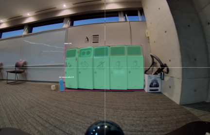
Fig. 4. Object detection and segmentation pipeline. GroundingDINO detects objects from text prompts (e.g., “bottle,” “trash bins”) and produces bounding boxes, which SAM refines into pixel-level masks. Segmentation constrains the association of image-projected LiDAR points to the object region, improving 3D anchoring accuracy.
3.4.2. Stage 2: Instance Segmentation Refinement
To improve the spatial precision of semantic evidence, we refine bounding boxes with pixel-level instance masks using the SAM or its lightweight variant MobileSAM 28,29. The reported configuration uses MobileSAM 29 with the vit_t TinyViT image encoder (\(\approx 5.78\)M parameters; \(\approx 9.66\)M for the full model), which is trained by decoupled distillation from the original SAM ViT-H and is reported to be more than \(60\times\) smaller than the original SAM at near-parity mask quality on standard benchmarks. SAM’s zero-shot ability to produce accurate masks for novel object types 28 enables the robot to isolate arbitrary landmarks (e.g., unusual furniture, decorative objects) on the map without requiring category-specific training. Each bounding box \(b_i\) serves as a prompt to SAM, which produces a binary mask \(M_i\) delineating the object’s spatial extent. Masks suppress background clutter and improve the accuracy of associating image-projected LiDAR points to the object region. We use SAM exclusively as a box-prompted segmenter rather than as an automatic mask generator. The image encoder is invoked once per frame to cache image embeddings; the prompt encoder and mask decoder are then re-executed per box, reusing the cached embedding so that segmenting all detected boxes in a frame is dominated by the single encoder pass rather than by the per-box decoder calls.
3.4.3. Stage 3: Calibrated Label Rerank
Open-vocabulary detectors are prone to confusing visually similar classes (e.g., trash bin versus cardboard box, or chair versus armless chair), and the raw GroundingDINO label string is in general not constrained to the scene vocabulary. The STCM configuration therefore inserts a calibrated rerank stage between segmentation and metric grounding, implemented with a separate frozen CLIP ViT-B/32 vision–language encoder 46. For every canonical class \(c \in \mathcal{C}\), the rerank-alias text bank is encoded once at startup with the CLIP text tower and \(L_2\)-normalised, yielding a set \(\mathcal{F}^{\text{txt}}_c \subset \mathbb{R}^d\) of text features per class. Per-class scoring uses the maximum cosine similarity over that alias bank, so adding paraphrases broadens the receptive field of the rerank without diluting any single anchor phrase. At each frame the global image \(I_{\text{rgb}}\) is encoded once with the CLIP vision tower to produce an image feature \(\boldsymbol{f}^{\text{img}} \in \mathbb{R}^d\), and an image-level prior is computed for every label as
3.4.4. Stage 4: Metric Grounding via Image-Projected 3D LiDAR (with Optional Depth Fallback)
For each detected object \(i\), we estimate its 3D position by intersecting the detection mask \(M_i\) with a LiDAR point cloud that has been projected into the image frame. At time \(t\), the robot publishes a point cloud message in which each point carries both its 3D coordinates \(\boldsymbol{p}_j^{\text{lidar}}=(x_j,y_j,z_j)\) expressed in lidar_link and its corresponding image coordinates \(\boldsymbol{u}_j=(u_j,v_j)\) [pixel]. We select the subset of LiDAR points whose projections fall inside the segmentation mask as in Eq. (11):
When no projected LiDAR points fall inside \(M_i\) (e.g., due to sparsity or occlusion), we optionally use a monocular depth estimator (Depth Anything 44) to obtain a dense depth map and back-project pixels in \(M_i\) to a 3D estimate. In the on-robot configuration evaluated here, this monocular fallback is explicitly disabled and detections whose mask carries no projected LiDAR hit are dropped, so all reported scene-level metrics in Section 5.3 are derived from LiDAR-anchored detections only. The fallback mechanism is thus not required for the core STCM pipeline.
Depth-only variant for public RGB-D benchmarking.
For the public-benchmark evaluation on NYUv2 (Section 5.5), the deployed fisheye+LiDAR pipeline cannot be executed because NYUv2 contains only single-view Kinect RGB-D images and provides no LiDAR return. To still place STCM’s perception subroutine on a recognized public RGB-D benchmark, we evaluate a depth-only variant of the open-vocabulary subroutine, denoted STCM-Depth, in which the registered Kinect depth channel substitutes for image-projected LiDAR as the geometric anchor that constrains mask–3D association and feeds a gravity-aligned plane prior. The depth map is back-projected per pixel using the Kinect intrinsics, and per-pixel surface normals are computed by central differences on the back-projected points; the projection of each normal onto the gravity-up vector \(\boldsymbol{u}=[0,-1,0]^\top\) in the camera frame is denoted \(u_{\text{proj}}\). Greedy RANSAC over the back-projected cloud then fits up to three dominant planes: in each round, \(200\) iterations of three-point fits compete for inlier sets within a perpendicular distance of \(0.04\) m, the winning plane is refined by singular-value decomposition over its inliers, its inliers are removed, and the procedure repeats up to a hard cap of three planes or until fewer than \(4000\) inliers remain. Each refined plane is then classified by combining \(u_{\text{proj}}\) and the mean image-row coordinate of its inliers: planes with \(u_{\text{proj}}>0.7\) and mean row below \(0.4H\) are tagged floor, planes with \(u_{\text{proj}}<-0.7\) and mean row above \(0.35H\) are tagged ceiling, planes with \(|u_{\text{proj}}|<0.3\) are tagged wall, and the residual is tagged other. The depth-only NYUv2 rasterisation then proceeds in three phases: instance-class candidates from GroundingDINO + MobileSAM + CLIP rerank are painted into the semantic map in descending order of fused score (Phase A); the floor, ceiling and wall masks from the plane classifier are then assigned to still-unlabelled pixels under fixed structural priors (Phase B); and any remaining pixels are filled by next-best candidate and dense-CLIP residuals (Phase C). Plane consensus therefore acts only on the structural-class subset and does not rerank instance-class detections. All other modules (GroundingDINO + MobileSAM detection, prompt bank, label rerank) are unchanged from Stages 1–3. The NYUv2 numbers in Table 8 (in Section 5.5) therefore characterize the depth-anchored open-vocabulary perception module of STCM, not the full LiDAR-fused system; we report them alongside supervised RGB-D upper bounds rather than as a like-for-like benchmark of the deployed pipeline.
3.4.5. Stage 5: Map-Frame Observation Output
Because Stage 4 already produces \(\boldsymbol{p}_i^{\text{map}}\) directly by composing the ROS 2 TF tree (whose parent \(\rightarrow\) child ordering is map \(\rightarrow\) odom \(\rightarrow\) base_footprint \(\rightarrow\) base_link \(\rightarrow\) lidar_link) into the single map-from-lidar transform \(\boldsymbol{T}_{\text{map}\leftarrow\text{lidar}}\) that is applied to each LiDAR-frame point, no additional rigid-body transform is applied at this stage; Stage 5 only assembles the per-frame observation set used by downstream fusion. For each accepted detection \(i\) at time \(t\), the rerank label \(l_i\), the map-frame anchor \(\boldsymbol{p}_i^{\text{map}}\) from Stage 4, and the fused confidence \(c_i\) from Stage 3 are emitted as
3.4.6. Stage 6: Fusion into STCM Place Graph
Semantic evidence is accumulated into the place nodes identified by GNG. At time \(t\), the winner node \(i^*\) has been determined from the robot’s position. We construct a semantic observation vector \(\boldsymbol{o}_t \in \mathbb{R}^{|\mathcal{C}|}\) where each component \(o_{t,c}\) aggregates confidence for class \(c\) from detections in \(\mathcal{O}_t\). In our default deployment, we use max aggregation: when multiple detections with label \(c\) are present at time \(t\), we set \(o_{t,c} = \max_{j: l_j=c} c_j\), i.e., the maximum confidence among all detections of class \(c\) in \(\mathcal{O}_t\). If no detection with label \(c\) is present, \(o_{t,c}=0\) (the system also supports sum aggregation via the place_gng_semantic_aggregation parameter, but max is the default).
The node’s semantic score vector \(\boldsymbol{s}_{i^*}\) is updated using exponential smoothing as in Eq. (13):
Optionally, we can also store the metric anchors \(\{\boldsymbol{p}_i^{\text{map}}\}\) as object-level landmarks associated with the place node, enabling finer-grained spatial queries and affordance reasoning.
3.5. Instance-Level GNG for Semantic Object Management
While place-level GNG (Section 3.3) discovers topological nodes from robot trajectories, the semantic layer must also distinguish multiple instances of the same object class. For example, a corridor may contain multiple chairs, tables, or doors. Simple distance-based merging (checking if a new detection is within a fixed radius of existing detections) suffers from two problems: (1) threshold sensitivity, where too large a threshold causes distant instances to merge incorrectly and too small a threshold causes the same object to create duplicates under localization drift; (2) lack of adaptability, since static thresholds cannot handle object scale variation or evolving spatial distributions.
To address this, we employ a second GNG module operating at the instance level: for each semantic class \(c \in \mathcal{C}\), we maintain a separate incremental GNG model \(\text{GNG}_c\) that clusters observed object positions into distinct instance prototypes. This instance-level GNG provides adaptive, incremental clustering that learns the spatial distribution of each object class during the mapping pass and naturally handles revisits, localization uncertainty, and scale variation.
3.5.1. Per-Label Instance Clustering
For each semantic class \(c\), we maintain a GNG model \(\text{GNG}_c = (\mathcal{I}_c, \mathcal{E}_c)\), where \(\mathcal{I}_c\) is the set of instance prototype nodes and \(\mathcal{E}_c\) is the set of instance association edges. Each instance node \(\iota_j \in \mathcal{I}_c\) is characterized by three attributes: a prototype position \(\boldsymbol{m}_j \in \mathbb{R}^3\) representing the 3D location in the map frame, an observation count \(\eta_j\) tracking the number of detections associated with this instance, and an accumulated confidence \(\phi_j\) that sums the detection confidences over all observations.
When a new detection \((l, \boldsymbol{p}^{\text{map}}, \gamma)\) arrives with label \(l = c\) and confidence \(\gamma\), we present its map-frame position \(\boldsymbol{p}^{\text{map}}\) to \(\text{GNG}_c\). The GNG algorithm proceeds as follows (illustrated in Fig. 5).
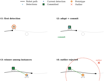
Fig. 5. Instance-level GNG illustration. As the robot moves, repeated detections of the same object arrive with small positional variation. The winner prototype adapts toward consistent observations, while detections that fall beyond the gating distance are rejected as outliers when the gate is active. This sequential filtering yields stable instance prototypes despite noise and revisits.
Step 1: Outlier gating. To prevent spurious detections from corrupting the instance set, we first check whether the new position is within a gate distance \(D_{\text{gate}}\) of an existing instance. When \(\mathcal{I}_c\) is nonempty, the nearest-instance distance is
Step 2: Winner selection. Compute distances to all instance prototypes as in Eq. (17):
Step 3: Prototype adaptation. The winner prototype is adapted toward the new observation as in Eq. (19):
Step 4: Edge creation and aging. An edge between \(j^*\) and \(j_2\) is created or refreshed as in Eq. (21):
Step 5: Node insertion. If the winner distance exceeds a creation threshold \(D_{\text{new}}^{\text{inst}}\), a new instance node is created as in Eq. (22):
Step 6: Commitment to semantic graph. Instance nodes are committed to the STCM semantic graph only after accumulating a minimum number of observations \(\eta_{\min}\) (typically 3–5). This filters transient detections and ensures that graph nodes represent stable, repeatedly observed objects. When \(\eta_j \geq \eta_{\min}\) and the instance is not yet in the graph, a new graph node is created with label \(c\), position \(\boldsymbol{m}_j\), and initial confidence \(\phi_j / \eta_j\). In the reported configuration \(\eta_{\min}=3\).
Initialisation, warm-up, and instance identity. The per-update primitive of Steps 1–6 is wrapped by a two-regime identity resolver. For each class \(c\) the first detection lazily instantiates a dedicated instance-GNG \(\text{GNG}_c\). During a warm-up window—until \(\max(2\lambda,20)\) detections accumulate, where \(\lambda\) is the GNG insertion interval—the GNG winner rule is bypassed and instances are formed by distance-based clustering: a detection is merged into an existing instance within the instance merge distance \(d_{\text{merge}}\) and otherwise seeds a new one. Once warm, instance identity is read from the connected components of \(\text{GNG}_c\), with the nearest-component test replacing the single-winner rule; the per-class winner–second-nearest edges of Step 4 exist only after the backend has been seeded with two prototypes. This warm-up is the instance-level counterpart of the two-prototype cold-start used by the place graph.
3.5.2. Cross-Label Merge and Label-Switch Hysteresis
The per-class instance stream of Steps 1–6 is duplication-robust within a single label but cannot, by itself, prevent the open-vocabulary detector from spawning twin instances when the same physical object alternates between two near-synonyms across frames (for example, a single office chair detected as “chair” from one viewpoint and as “armless chair” from another). Two cross-class adjudication mechanisms specific to the STCM backend close this gap by re-using the calibrated outputs of Stage 3. First, an appearance-aware cross-label merge compares each incoming detection against currently resolved instance labels in a neighbourhood radius. Let \(r_{\text{cl}}\) denote the cross-label merge distance and let \(\boldsymbol{e}_i\) denote the CLIP crop feature returned with detection \(i\) from Stage 3. Whenever the detection’s resolved label differs from the resolved label of an existing instance \(\iota_j\) but their centroids satisfy \(\|\boldsymbol{p}^{\text{map}}-\boldsymbol{m}_j\|\leq r_{\text{cl}}\), the manager checks the cosine similarity between \(\boldsymbol{e}_i\) and the running appearance descriptor \(\bar{\boldsymbol{e}}_j\) of \(\iota_j\); if \(\cos(\boldsymbol{e}_i,\bar{\boldsymbol{e}}_j)\geq\rho_{\text{cl}}\), the detection is absorbed into \(\iota_j\) rather than instantiating a fresh node under the new label, and its label-score map contributes to a running vote tally on \(\iota_j\) instead of duplicating geometry. The reported configuration uses \(r_{\text{cl}}=0.6\) m and \(\rho_{\text{cl}}=0.25\). Second, a label-switch hysteresis controls how the resolved label of \(\iota_j\) may flip once a cross-label merge succeeds: a candidate replacement label is accepted only when its margin over the current label exceeds \(\delta_{\text{lab}}=0.15\) in vote score and it has been observed consecutively in the merge stream at least \(K_{\text{lab}}=2\) times. This prevents single noisy rerank decisions from flipping a long-supported instance label and stabilises the dominant class assigned to each STCM graph node. The combined cross-label merge and hysteresis path is the principal duplicate-suppression mechanism reported in the perception-backend variant comparison of Table 5 (in Section 5.3).
3.5.3. Integration with Place Graph
The instance-level GNG operates independently from the place-level GNG but shares the same map frame. Both modules consume the same map-frame semantic observations from \(\mathcal{O}_t\). Place-node semantic scores are updated directly from per-frame observations using the detection-level aggregation described in Section 3.4.6, while the instance manager separately consolidates those observations into persistent object instances. In the default configuration, place-score fusion uses max aggregation over detections with the same label, followed by exponential smoothing; sum aggregation is also supported through the place_gng_semantic_aggregation parameter. Instance prototypes are associated with the STCM graph for object-level queries and inspection, but they are not used as the default source for updating place-node semantic score vectors.
3.6. STCM Graph Representation and Output
The STCM graph \(G = (V, E)\) is the central data structure for task planning and human-robot communication. The complete formalization is given in Eq. (24):
Each node \(v_i \in V\) represents a place characterized by four principal attributes. The position \(\boldsymbol{r}_i \in \mathbb{R}^2\) encodes the representative 2D coordinates of the place in the map frame, serving as the navigational target. The semantic scores \(\boldsymbol{s}_i \in [0,1]^{|\mathcal{C}|}\) store accumulated confidence values for each semantic class in \(\mathcal{C}\), where the normalisation to \([0,1]\) is inherited from the per-frame observation vector \(\boldsymbol{o}_t\) and the exponential-smoothing update of Eq. (13); each class is updated independently and the components are not constrained to sum to unity. The label \(\ell_i\) denotes the dominant observed semantic class for the place, determined by the highest-scoring element of \(\boldsymbol{s}_i\); in the present pipeline this dominant cue is object-derived (e.g., “trash bin,” “water fountain,” “meeting table set”) and is exposed to the language interface as a dominant semantic cue rather than as a curated place category. Coarser place categories such as “kitchen,” “bedside,” or “doorway” would require a separate place-type inference step over \(\boldsymbol{s}_i\) and the local object distribution, which is left to future work. Finally, the visit count \(n_i\) records the number of times the node was selected as the winner during GNG updates, providing a measure of node stability and observational support.
Each edge \(e_{ij} \in E\) represents a proximity relation, an observed traversal relation, or both, with optional attributes such as traversal count or traversal cost.
The STCM graph provides outputs for planning, inspection, and explainability. We export the graph as a NetworkX graph object, as a JSON file (stcm.json), and as ROS 2 topics (/semantic_graph/nodes, /semantic_graph/place_graph) for real-time visualization in RViz. Each node contains id (unique identifier), label (semantic class), pose (\(x\), \(y\) coordinates), scores (confidence values for all \(|\mathcal{C}|\) semantic classes), and visits (observation count). Each edge contains source and target node IDs, traversals (transition count), and age (edge age for pruning). Exposing the node scores vector provides the evidence behind the dominant cue (e.g., co-occurrence of high “sink” and “stove” scores would motivate a future place-category step that lifts the node to a “kitchen” label), enabling transparent reasoning about place assignments.
The graph is serialized to JSON for storage, visualization, and interfacing with external systems. A sample node in JSON format is as follows:
{
  "id": "place_12",
  "label": "water fountain",
  "pose": [2.34, -1.12],
  "scores": {"water fountain": 0.71,
             "trash bin": 0.18, "chair": 0.06},
  "visits": 47
}
The scores field contains confidence values for all configured semantic classes; only non-zero scores are shown above for brevity. Classes not observed at a node are stored as zero, and the exponential-smoothing update (Eq. (13)) decays a class’s accumulated score on every frame in which it is absent (\(o_{t,c}=0\)). In the reported configuration, label is the dominant object/landmark cue (the \(\mathop{\rm arg~max}\limits\) of scores), not a room-level place category such as “kitchen.”
The same artefact also lists grounded object instances and their nearest-place associations. A representative entry of the LLM-facing objects list and the corresponding object_place_links record are as follows:
{ "id": "bottle_inst_0",
  "label": "bottle",
  "pose": [10.15, 0.76, 0.03],
  "stability": 1.0 }

{ "object_id": "bottle_inst_0",
  "place_id": "place_22",
  "distance": 1.53 }
Optional per-object keys (caption, dimensions, heading) appear only when populated. Object–place relations are stored as nearest-place link records (nearest place by 2D Euclidean distance) rather than as typed edges; the serialized graph edges are place–place connections (with source, target, traversals, and age), while object–object edges are not exported.
The canonical output of STCM is the serialized graph file stcm.json, which constitutes the structured interface between perception, planning, and language grounding. The same JSON payload is consumed by two downstream consumers without modification: the ROS 2 stack ingests it to recover place nodes, object instances, and edges for graph-based planning and Nav2 waypoint resolution, and the LLM grounder fetches it (in full or as a node/object subset projection) as in-context evidence for mapping a natural-language command to a target node identifier. Because the LLM operates on this JSON rather than on raw sensor streams, the language-to-graph step is decoupled from perception and from low-level control: the LLM emits only graph-referenced goals, while metric planning and execution remain the responsibility of graph search and Nav2 (Section 3.8). This file-level interface also makes the representation portable across sessions and inspectable offline, which is exploited in the evaluation by replaying the same stcm.json under the LLM and the no-LLM template baselines on identical command sets (Section 5.4).
3.8. LLM-Based Language Grounding and Planning
For complex natural language instructions that involve spatial reasoning (e.g., “go to the table between the two chairs” or “navigate to the smallest chair near the door”), we extend STCM with an LLM-based planning interface built on LangChain and LangGraph. The LLM serves as a high-level planner that grounds language commands in the STCM object graph and generates navigation sequences, while graph search and Nav2 remain responsible for execution.
The system provides the LLM with a structured representation of the environment: a list of detected objects from the STCM graph, each with an identifier, semantic label, map-frame centroid, accumulated confidence, and an optional axis-aligned 2D extent in the map frame derived from the projected LiDAR support of Section 3.4 when available. The LLM is equipped with a toolbox of spatial reasoning functions including find_near(target, anchor), find_between(target, anchor1, anchor2), find_left(target, anchor), find_right(target, anchor), and ordering tools such as order_left_to_right(target) and order_smallest_to_largest(target). Left/right predicates are resolved viewpoint-relative to the robot’s most recent base-link pose, which is supplied to the LLM alongside the object table; order_smallest_to_largest consumes the optional 2D extent field when populated and otherwise returns an explicit “size unavailable” error rather than fabricating an ordering. These tools implement geometric predicates using object centroids, the optional extent field, and viewpoint-relative spatial relations, providing symbolic abstractions over the metric map.
Given a natural language command, the LLM generates a sequence of tool calls to resolve spatial references, followed by a final command_robot(list_of_commands) call specifying navigation primitives: go_near(object_id) or go_between(object_id1, object_id2). For example, the instruction “go to the second chair from the left near the table” is decomposed into: (1) find_near(‘‘chair,’’ ‘‘table’’) to identify chairs near tables, (2) order_left_to_right(‘‘chair’’) to rank them spatially, (3) select the second ID, and (4) command_robot([‘‘go_near,’’ [id]]). An optional critic-LLM review path allows a second LLM to review the reasoning trace and provide corrective feedback before execution (this is a two-LLM review pipeline, not a reinforcement-learning actor–critic).
The output navigation commands reference object IDs in the STCM graph. These are resolved to metric waypoints via the object centroids \(\{\boldsymbol{p}_i^{\text{map}}\}\) or place node positions \(\{\boldsymbol{r}_i\}\), which are then executed by Nav2. This design aligns with recent findings that augmenting LLM prompts with an extracted entity–relation graph structure can improve spatial reasoning in path-planning tasks 31, while keeping metric planning and control separate ensures safety and ROS 2 compatibility. The LLM interface enables flexible language-driven interaction without requiring end-to-end learning or custom low-level controllers.
4. Implementation and Experimental Setup
4.1. Robot Platform
We have developed the Ranger Garden Assistant mobile robot platform as an integrated system for assistive navigation research. The complete ROS 2 software stack, including hardware integration packages, sensor drivers, SLAM configurations, and navigation parameter files, is made publicly available to support reproducibility and future research at https://github.com/anh0001/ranger-garden-assistant. We implement and evaluate STCM on this platform, shown in Fig. 6. The platform is built upon an AgileX Ranger Mini 3.0 omnidirectional base equipped with sensing and manipulation hardware for outdoor and indoor assistive tasks. The robot’s computing platform runs Ubuntu 22.04 with ROS 2 Humble, providing the middleware foundation for sensor integration, navigation, and system coordination.
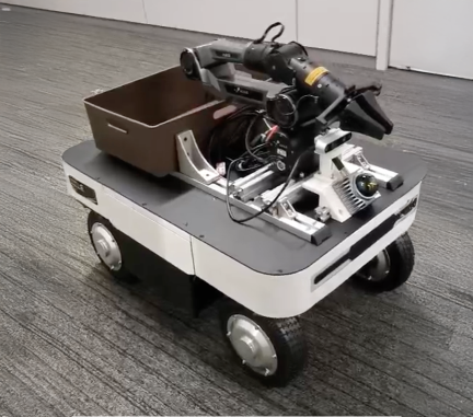
Fig. 6. Ranger Garden Assistant mobile robot platform. The system integrates an AgileX Ranger Mini 3.0 omnidirectional base, Livox Mid-360 3D LiDAR, Tier IV C2-176 fisheye camera (176° FOV), and AgileX PiPER 6-DOF robotic arm, running ROS 2 Humble with Navigation2 and FAST-LIO2.
The mobile base employs an AgileX Ranger Mini 3.0 omnidirectional drive system with swivel wheels on each corner, enabling lateral motion and in-place rotation essential for maneuvering in constrained indoor spaces. This omnidirectional capability allows the robot to adjust its orientation and position independently, facilitating navigation in narrow corridors and doorways typical of domestic environments. The base supports a maximum linear velocity of 0.26 m/s and angular velocity of 1.0 rad/s, values selected to balance navigation efficiency with safety in human-occupied spaces.
For 3D perception, the platform integrates a Livox Mid-360 3D LiDAR sensor with 360° horizontal field of view, detection range up to 70 m, and point rate of 200,000 points per second. The Mid-360 employs a non-repetitive scanning pattern that provides high-density coverage over time, a characteristic particularly beneficial for both SLAM and semantic mapping. Unlike conventional mechanical LiDARs that repeat the same scan lines, the Livox Mid-360’s quasi-random pattern accumulates dense 3D geometry as the sensor moves, ensuring that the entire 360° environment is thoroughly sampled even during short observation periods. This high point density and wide coverage make the Mid-360 well-suited for STCM’s dual requirements of precise metric localization and accurate semantic anchoring via LiDAR-to-camera projection.
box_threshold is reported with sensitivity in Section 4.2.| Module | Parameter | Value | Rationale |
| Place GNG | \(D_{\text{new}}\) (node creation) | 0.5 m | Indoor place granularity 26 |
| \(\epsilon_b\) (winner learn rate) | 0.1 | Standard GNG 25 | |
| \(\epsilon_n\) (neighbor learn rate) | 0.01 | Ratio \(\epsilon_b/\epsilon_n=10\) 25 | |
| \(a_{\max}\) (edge age threshold) | 50 | Empirical, place-traversal scale | |
| Instance GNG | \(D_{\text{new}}^{\text{inst}}\) (instance creation) | 0.5 m | Minimum inter-instance gap |
| \(\epsilon_w\) (winner learn rate) | 0.05 | Slower than place rate | |
| \(\epsilon_n^{\text{inst}}\) (neighbor learn rate) | 0.0006 | Conservative neighbour drift | |
| \(a_{\max}^{\text{inst}}\) (edge age) | 200 | Persistent object scale | |
| \(D_{\text{gate}}\) (outlier gate) | 0.0 m (disabled) | Accumulation absorbs noise | |
| \(\eta_{\min}\) (min. observations) | 3 | Commit-on-evidence threshold | |
| Semantics | \(\tau_{\text{box}}\) (box confidence) | 0.45 | Deployed STCM operating point, downstream CLIP rerank absorbs false positives |
| \(\tau_{\text{text}}\) (text matching) | 0.45 | Matched to \(\tau_{\text{box}}\) in the deployed configuration | |
| \(\alpha\) (temporal fusion rate) | 0.1 | \(\approx 10\)-visit time constant |
Visual perception is provided by a Tier IV C2-176 fisheye camera with 176° field of view, delivering wide-angle RGB imagery for semantic detection and multi-modal fusion. The fisheye lens captures substantially broader coverage than standard perspective cameras, enabling semantic detection of objects in peripheral regions that would otherwise require multiple viewpoints or active camera steering. This wide field of view is especially valuable in corridor and room-corner scenarios where landmarks may appear at large angles from the robot’s forward direction.
The platform also carries an AgileX PiPER 6-DOF robotic arm for future assistive manipulation; it is not exercised in the navigation experiments reported here. Communication between the computing platform and the drive and manipulator controllers is handled by two USB-CAN adapters.
The software stack is organized around ROS 2 Humble as the core middleware for sensor integration, navigation, and system coordination. FAST-LIO2 provides LiDAR-inertial odometry and mapping, delivering real-time pose estimation and metric map construction as described in Section 3.2. Navigation2 (Nav2) serves as the ROS 2 navigation stack for global and local planning, costmap management, and recovery behaviors, enabling the robot to execute waypoint sequences generated from STCM graph plans. MoveIt 2 is installed for future manipulation planning but is not used in the reported experiments. Finally, Octomap_server2 provides 3D occupancy mapping for visualization and collision checking, complementing the point cloud maps produced by FAST-LIO2 with volumetric representations suitable for display in RViz and offline analysis.
4.2. Parameter Configuration
Table 1 summarizes the parameter values used in our implementation, selected based on the spatial scale of the environment and empirical tuning. The GNG threshold \(D_{\text{new}} = 0.5\) m produces a fine-grained place graph with dense node coverage, resulting in approximately 60–80 place nodes for the 40-meter corridor. The semantic fusion rate \(\alpha = 0.1\) provides stable label accumulation while allowing adaptation to changing observations over roughly 10 visits to a place. Navigation uses Nav2 with Smac Planner 2D for global planning (0.05 m costmap resolution), MPPI controller for local trajectory optimization, maximum linear velocity 0.26 m/s, and maximum angular velocity 1.0 rad/s. Each parameter in Table 1 carries an explicit rationale column. Place- and instance-GNG learning rates and edge-age thresholds follow standard GNG-style ratios 25,26; spatial thresholds \(D_{\text{new}}\) and \(D_{\text{new}}^{\text{inst}}\) are matched to the indoor place granularity discussed in Section 3.3; the open-vocabulary detector thresholds \(\tau_{\text{box}}\) and \(\tau_{\text{text}}\) are inherited from GroundingDINO defaults 27; and the fusion rate \(\alpha\) is chosen to absorb roughly ten observations before saturation. The entry \(D_{\text{gate}} = 0.0\) m is explicitly noted to mean that the outlier gate is disabled in the reported runs, so all detections within the per-class instance space are admitted and the instance-GNG winner-take-all dynamics absorb spurious returns through accumulation rather than hard rejection.
box_threshold on the proposed STCM backend across the three recorded scenes. All other parameters held at the per-scenario defaults; mean \(\pm\) s.d. over \(n \geq 3\) replicated replays per threshold. The deployed STCM configuration uses \(\tau_{\text{box}}=\tau_{\text{text}}=0.45\) (not shown in the swept range); the values below characterize robustness across lower and moderate operating points.box_threshold |
Meeting (S1) | Living lab (S2) | Outdoor (S3) |
| \(0.25\) | 0.484\(\pm\)0.020 | 0.547\(\pm\)0.047 | 0.459\(\pm\)0.005 |
| \(0.30\) | 0.484\(\pm\)0.025 | 0.508\(\pm\)0.057 | 0.445\(\pm\)0.008 |
| \(0.35\) | 0.466\(\pm\)0.013 | 0.554\(\pm\)0.016 | 0.450\(\pm\)0.018 |
| \(0.40\) | 0.458\(\pm\)0.023 | 0.549\(\pm\)0.018 | 0.450\(\pm\)0.005 |
A compact sensitivity study was performed on the front-end knob that most directly governs detection quality: the GroundingDINO box-confidence threshold box_threshold. The deployed STCM configuration uses \(\tau_{\text{box}}=\tau_{\text{text}}=0.45\) as its reported operating point; to characterize robustness at lower and moderate detector thresholds, the proposed STCM backend was additionally swept over \(\{0.25, 0.30, 0.35, 0.40\}\) on all three recorded scenes (S1, S2, S3), with every other parameter held at the per-scenario default. The sweep should be interpreted as a robustness check on lower-threshold operating points rather than as alternative headline configurations, and extending the sweep to include the exact deployed \(0.45\) point is outside the scope of the present evaluation. Results are reported as object-graph \(F_1\) under Hungarian-matched \(1:1\) same-label scoring at the per-scene match radius (strict \(1.0\) m on S1/S2; outdoor per-class radius on S3), as mean \(\pm\) s.d. over \(n \geq 3\) replicated replays per threshold. The numerical sweep is reproduced in Table 2. STCM’s per-class CLIP rerank discharges false-positive responsibility downstream of the box-confidence gate, so the backend prefers a relatively loose threshold and is broadly flat across the swept lower-threshold range: the within-threshold spread is \(\leq 2.6\) pp on S1 (\(0.458\)–\(0.484\)), \(\leq 4.6\) pp on S2 (\(0.508\)–\(0.554\)), and \(\leq 1.4\) pp on S3 (\(0.445\)–\(0.459\)), all comparable to the replicate s.d. within a single threshold. Within this swept range, performance is essentially flat: the \(0.30\) probe ties the peak on S1 (\(0.484\)) and lies within \(0.046\) of peak on S2 and within \(0.014\) of peak on S3, indicating lower-threshold robustness of the front end under the evaluated replay protocol. The GNG-side knobs (\(D_{\text{new}}\), \(\alpha\), \(\eta_{\min}\)) were not swept and lie outside the scope of the present evaluation. A separate diagnostic pass identified GNG over-commit as the dominant false-positive source on outdoor data; raising the cross-label merge distance from \(0.45\) m to \(0.8\) m in the outdoor configuration lifted the outdoor \(F_1\) by \(+0.033\) absolute under per-class/alias scoring.
5. Experimental Results
The evaluation has been organized around the three-scenario protocol. We first describe the dataset and scoring protocol (Section 5.1), then report graph-feasibility navigation success and path-length ratios (Section 5.2), per-scene semantic-labelling accuracy as object-graph \(F_1\) together with a perception-backend variant comparison that isolates detector-bound from graph-bound failure modes (Section 5.3), the LLM ablation with paired McNemar tests (Section 5.4), the depth-only variant evaluated on NYUv2-40 (Section 5.5), per-module runtime and hardware (Section 5.6), and qualitative results (Sections 5.7–5.12).
| Scene | Storage | Duration [s] | Vocab. size | GT instances |
| meeting (S1) | sqlite3 | 175 | 10 | 20 |
| livinglab (S2) | mcap | 153 | 11 | 23 |
| outdoor_livinglab (S3) | mcap | 170 | 14 | 19 |
5.1. Dataset and Evaluation Protocol
Three recorded sessions are used, spanning a structured meeting room (S1), an indoor elderly-healthcare living lab (S2), and an outdoor extension of the same living lab (S3) treated as an out-of-distribution probe with respect to the indoor-tuned prompt bank. Because the S3 perception configuration (the outdoor aliases and the cross-label merge distance of Section 4.2) was adjusted after inspecting S3 outputs, the S3 result is reported throughout as a diagnostic alias-tuned probe rather than as a blind out-of-distribution generalisation test, whereas the S1 and S2 prompt phrasings were fixed before scoring. The dataset card is reproduced in Table 3, and three representative onboard frames per scene are shown in Fig. 7. The meeting session is a structured indoor space populated with ten standard indoor classes; the living-lab session is a workshop-style space configured for assistive-mobility and elderly-care evaluation, populated with both standard indoor furniture and assistive devices (electric wheelchair, vacuum cleaner, plant pots, shoes, small electric vehicle); the outdoor session shares the same site but exhibits only \(\sim 3\) classes of vocabulary overlap with the indoor sessions, so its \(14\)-class outdoor vocabulary stresses the indoor-tuned prompt bank. Each session is evaluated through deterministic offline replays with small box_threshold perturbations, so we report replay repeatability rather than random-seed independence. For each scenario we apply a shared protocol covering graph-feasibility navigation success rate and path-length ratio over \(15\) trials per run replicated across \(3\) runs per scene under box_threshold perturbation; semantic labelling accuracy as object-graph precision, recall, and \(F_1\) under Hungarian-matched \(1:1\) same-label scoring at the per-scene match radius; and natural-language grounding accuracy on \(45\) commands on S1 (\(10\) simple, \(10\) disambiguation, \(10\) compositional, \(15\) functional/intent), a parallel \(30\)-command set on S2 (\(5/5/5/15\)), and a matched \(30\)-command set on S3.
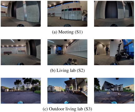
Fig. 7. Three representative onboard frames per scene illustrate the visual diversity of the S1/S2/S3 sessions in Table 3.
Per-scene class inventories are: S1 meeting: bench, bottle, cardboard box, chair, cup, door, emergency exit sign, meeting table set, trash bin, water fountain; S2 living-lab: bench, cardboard box, chair, door, electric vehicle, large power bank, meeting table set, plant pot, shoes, trash bin, vacuum cleaner; S3 outdoor living-lab: basketball, cardboard box, chair, electric scooter, electric utility vehicle, electric wheelchair, pair of ramps, portable power station, prohibition sign, rectangular table, traffic cone, trailer, trolley, umbrella.
Ground-truth object poses were obtained by manual in-situ annotation during the rosbag recording sessions rather than by post-hoc projection from the constructed map. For each scene, every object in the per-scene class inventory was measured in meters on the floor plane against a fixed scene origin coincident with the robot start pose, using a hand-held tape measure for in-plane \((x, y)\) position and recording the class label alongside each measurement. The resulting per-scene annotation tables list one row per physical object instance and serve as the reference set \(S_{GT}\) used for the Hungarian-matched object-graph precision, recall, and \(F_1\) scoring (Section 5.3), the within-radius checks of the graph-feasibility navigation protocol (Section 5.2), and the semantic cardinality deviation \(|\Delta S|/|S_{GT}|\) reported in the dual-GNG ablation (Table 11 in Section 5.8). Because the annotation is metric and class-labelled but not orientation-resolved, the scoring contracts use position-only \(1:1\) matching at the per-scene match radius and do not rely on bounding-box overlap.
5.3. Semantic-Labelling Accuracy and Perception-Backend Variant Comparison
Semantic-labelling accuracy is reported as object-graph precision, recall, and \(F_1\) under Hungarian-matched \(1:1\) same-label scoring at the per-scene match radius (strict \(1.0\) m and no-alias contract on the indoor scenes; outdoor per-class radius with post-hoc-tuned aliases on S3). To clarify the role of ground-truth annotation in prompt design: per-scene class inventories were known to the operator before deployment as “scenario task vocabulary” (the kinds of objects the assistive robot is expected to encounter in a meeting room, a living lab, or its outdoor extension); the predeclared scenario-vocabulary prompt phrasings reuse those class names and naive paraphrases of them (plurals, stripped modifiers), were fixed before scoring, and do not consume per-instance ground-truth locations or counts, and instance positions in \(S_{GT}\) are used only for downstream Hungarian matching, not to construct prompts. The headline backend (denoted “STCM”; predeclared scenario-vocabulary prompt phrasings, no semantic prior) reaches \(F_1=0.449\)\(\pm\)0.037 on S1 (\(n=3\); tied within \(1\sigma\) with the prior STCM-nyu40 cell at 0.458\(\pm\)0.127 but with approximately threefold tighter run-to-run spread), 0.535\(\pm\)0.028 on S2 (\(n=3\); \(+0.061\) above the strongest prior-augmented variant STCM+ESANet at \(0.474\)\(\pm\)0.052), and 0.456\(\pm\)0.005 on S3 under the outdoor per-class radius and alias scoring contract (\(n=3\); \(+0.037\) above STCM+ESANet at 0.419\(\pm\)0.004, Welch \(t \approx 10.0\), \(p < 0.001\) with two-sided Welch–Satterthwaite degrees of freedom \(\approx 3.8\)). The macro mean of the three headline cells is \(F_1 =0.480\) for the STCM backend versus \(0.404\) for the strongest prior-augmented variant and \(0.388\) for the transformer-prior variant; the full per-backend table is given in Table 5 below. Under the strict global \(1.0\) m no-alias indoor contract used for S1 and S2, the earlier STCM-nyu40 outdoor three-run set scores \(F_1 =0.264\)\(\pm\)0.021, which we attribute to detector-bound rather than graph-bound errors; swapping the perception front end (analyzed below) improves S2 without modifying any STCM graph component.
To isolate detector-bound from graph-bound failure modes, we hold the STCM graph components (place-GNG, instance-GNG, LiDAR–image association, temporal score fusion, scoring harness) fixed and swap only the perception front end across five variants on all three scenes (S1, S2, S3). The variants are: the vanilla GroundingDINO-tiny + MobileSAM baseline; STCM-nyu40, which uses NYU-grounded prompt banks; STCM-Trans, which augments STCM-nyu40 with the per-pixel semantic prior produced by the transformer-based RGB-D segmenter of Section 5.5; STCM+ESANet prior, which substitutes an ESANet prior for the transformer prior; and the proposed STCM backend, which uses predeclared scenario-vocabulary prompt phrasings (with post-hoc-tuned aliases on S3, evaluated as a diagnostic probe) and no semantic prior. Cells are precision, recall, and \(F_1\) under Hungarian-matched \(1:1\) same-label scoring at the per-scene match radius (strict \(1.0\) m on S1/S2; outdoor per-class radius on S3); mean \(\pm\) s.d. over \(n\) replicated replays, with \(n \geq 3\) except where flagged.
Table 5 reports the result. Because the variants differ in detector checkpoint, CLIP rerank, prompt vocabulary, and prior simultaneously (see the table footnote), each row is read as a complete backend rather than as an isolated single-factor ablation. On S1 the STCM-nyu40 backend (GDINO-base + CLIP rerank + NYU-40 prompt bank) lifts \(F_1\) by \(+0.10\) over the vanilla GDINO-tiny baseline (\(0.362 \to 0.458\)), driven by both precision and recall; this end-to-end gain combines the larger detector checkpoint, the rerank stage, and the prompt bank and is not attributable to the prompt bank alone. Under \(n \geq 3\) replication, adding a per-pixel semantic prior on S1 reduces performance: STCM-Trans falls to 0.381\(\pm\)0.069 and STCM+ESANet prior to 0.320\(\pm\)0.087, both below the prior-free STCM-nyu40 mean. These replicated numbers reverse the direction of an earlier single-run pilot (values of \(0.444\) and \(0.421\)) that lay on the lucky end of the threshold sweep, which is the reason the ranking is now reported only over \(n \geq 3\) replicates. Under replication the priors are detrimental on S1, consistent with the prompt bank already saturating the S1 detection ceiling.
On S2 the trend reverses. Plain STCM-nyu40 sits at \(0.301 \pm 0.223\), below the vanilla mean of 0.411\(\pm\)0.047, because S2 contains assistive- and healthcare-context classes (electric vehicle, large power bank, shoes) that lie outside the NYUv2-indoor-furniture prompt bank’s training distribution. Adding a semantic prior closes this gap and exceeds the vanilla baseline under replicated scoring: STCM-Trans lifts S2 to 0.417\(\pm\)0.037 (matches the vanilla mean within one standard deviation; \(+0.12\) over plain STCM-nyu40), and STCM+ESANet prior lifts it to 0.474\(\pm\)0.052, the highest prior-augmented mean on S2. The STCM+ESANet-prior versus vanilla gap is \(+0.06\) in absolute terms, approximately \(1.4\sigma\) when pooled, which is suggestive but not conclusive at \(n = 3\) per cell.
| Partition | Arm | Top-1 | 95% CI | \(\boldsymbol{\Delta}\) | CI (\(\boldsymbol{\Delta}\)) | McNemar \(\boldsymbol{p}\) | \(\boldsymbol{b/c}\) |
| Spatial (\(n=30\)) | no-LLM (template) | \(0.433\) | \([0.27, 0.61]\) | — | — | — | — |
| Spatial (\(n=30\)) | +intent-lexicon | \(0.433\) | \([0.27, 0.61]\) | — | — | — | — |
| Spatial (\(n=30\)) | +LLM | \(0.433\) | \([0.27, 0.61]\) | \(+0.000\) | \([-0.09, 0.09]\) | \(1.000\) | \(1/1\) |
| Functional (\(n=15\)) | no-LLM (template) | \(0.000\) | \([0.00, 0.20]\) | — | — | — | — |
| Functional (\(n=15\)) | +intent-lexicon | \(0.333\) | \([0.15, 0.58]\) | \(+0.333\) | \([0.10, 0.57]\) | \(0.0625\) | \(5/0\) |
| Functional (\(n=15\)) | +LLM | \(\mathbf{0.600}\) | \([0.36, 0.80]\) | \(\mathbf{+0.600}\) | \([0.35, 0.85]\) | \(\mathbf{0.0039}\) | \(9/0\) |
| Eligible (\(n=39\)) | no-LLM (template) | \(0.333\) | \([0.21, 0.49]\) | — | — | — | — |
| Eligible (\(n=39\)) | +intent-lexicon | \(0.462\) | \([0.32, 0.61]\) | \(+0.128\) | \([0.02, 0.23]\) | \(0.0625\) | \(5/0\) |
| Eligible (\(n=39\)) | +LLM | \(0.564\) | \([0.41, 0.71]\) | \(+0.231\) | \([0.08, 0.38]\) | \(0.0117\) | \(10/1\) |
The proposed STCM backend reaches the highest observed macro-mean \(F_1\) across the three scenes (macro-mean \(0.480\) versus \(0.404\) for the strongest prior-augmented variant) and the highest per-scene mean on S2 and S3. The STCM variant replaces the curated NYU alias engineering with predeclared scenario-vocabulary prompt phrasings; under \(n = 3\) replicated scoring it is the highest-mean cell on the S2 and S3 columns, while on S1 STCM (0.449\(\pm\)0.037) and STCM-nyu40 (0.458\(\pm\)0.127) lie within one standard deviation of each other, with STCM offering materially tighter run-to-run dispersion. S1 \(F_1=0.449\)\(\pm\)\(0.037\) (\(+0.068\) over STCM-Trans and \(+0.129\) over STCM+ESANet prior); S2 \(F_1=0.535\)\(\pm\)\(0.028\) (\(+0.061\) over STCM+ESANet prior, outside that variant’s \(\sigma = 0.052\) band); and S3 \(F_1=0.456\)\(\pm\) \(0.005\) under outdoor per-class scoring (\(+0.037\) over STCM+ESANet prior; Welch \(t \approx 10.0\), \(p < 10^{-4}\) at \(n = 3\) per cell). Run-to-run dispersion is materially tighter as well (\(\sigma \leq 0.037\) versus \(\sigma \leq 0.087\) for the prior-augmented variants). On scenes whose vocabulary is well covered by GroundingDINO under the predeclared scenario-vocabulary phrasings, the STCM prompt bank can replace the semantic prior and yields higher means than the prior-augmented variants. On outdoor scenes, where geometric reach limits recall on far or sparse objects, STCM remains the strongest variant, and the residual gap on a handful of classes (trailer, rectangular table, trolley) suggests that semantic priors may complement the prompt bank in future work. Among the prior-augmented variants, STCM+ESANet prior outperforms STCM-Trans on S2 and S3 in mean (\(0.474\) vs. \(0.417\) on S2; \(0.419\) vs. \(0.367\) on S3), while STCM-Trans outperforms STCM+ESANet prior on S1 (\(0.381\) vs. \(0.320\)); the two prior-augmented variants are therefore reported as scene-dependent alternatives rather than as uniformly dominant backends.
5.4. LLM Ablation with Paired McNemar Analysis
The LLM in STCM performs language-to-graph grounding and to isolate the LLM’s contribution from spatial grounding, three arms are compared on the same predicted graph and the same command set: (i) a no-LLM deterministic template grounder, identical to the spatial grounder used in the baseline system; (ii) the same template augmented with an intent lexicon, a small deterministic regular-expression map of intent verbs to canonical labels; and (iii) the same template augmented with an LLM (Claude Sonnet 4.6, temperature \(0\), returns a ranked id list). Top-1 accuracy uses a \(1\) m spatial id-match fallback. We report paired top-\(1\) accuracy with \(95\%\) Wilson confidence intervals, the paired-discordant counts \((b, c)\) against the no-LLM template, and exact unadjusted two-sided McNemar \(p\)-values per subset in Table 6; the Holm-adjusted family-wise rate across the three subsets (Spatial, Functional, Eligible) preserves significance for the Functional (\(p_{\text{Holm}}=0.0117\)) and Eligible (\(p_{\text{Holm}}=0.0234\)) cells under the LLM arm (Spatial \(p_{\text{Holm}}=1.000\)). The functional/intent subset is the declared primary endpoint because it is answerable only by a system that can map intent to label; on these functional/intent commands the no-LLM template returns no candidate by construction, as it has no mapping from intent verbs to semantic labels. For two-scene combination on the perception-recoverable partition we additionally report a \(\sqrt{n}\)-weighted Stouffer combination and a stratified McNemar over pooled discordant counts as a sensitivity check; the per-scene discordant counts that feed the stratified combiner are reported in the running text below rather than tabulated separately because the S1 cell anchors the pre-declared paired analysis.
Table 6 reports the meeting scene result, on which the analysis was pre-declared. On the explicit spatial subset all three arms tie at \(0.433\) top-\(1\) accuracy (McNemar \(p = 1.000\), one discordant pair in each direction), so the deterministic spatial grounder already saturates this regime and the LLM is not responsible for system accuracy on commands such as “go to the chair nearest the door.” On the functional primary subset the LLM reaches \(0.600\) vs. \(0.000\) for the no-LLM template (\(\Delta = +0.60\), exact two-sided McNemar \(p = 0.0039\), \(b/c = 9/0\)); on the perception-eligible subset (commands whose gold referent is present in the predicted graph) the LLM still significantly outperforms the template (\(0.564\) vs. \(0.333\), \(\Delta = +0.23\), \(p = 0.0117\), \(b/c = 10/1\)), isolating ranker quality from perception confounds. Two-scene combination on the functional+recoverable partition (S1 meeting \(n=13\), \(b/c=9/0\); S2 living lab \(n=8\), \(b/c=5/0\)) gives Stouffer \(Z = 3.42\), \(p = 0.0006\) and stratified McNemar \(\sum_k b_k = 14\), \(\sum_k c_k = 0\), exact \(p = 0.0001\); the S2 stratum alone is not significant (exact \(p = 0.0625\)), so the combined significance derives from pooling with S1. The two combiners agree on direction and significance. The LLM also exceeds the small intent lexicon on the functional+recoverable subset (\(0.692\) vs. \(0.385\) on meeting; \(0.625\) vs. \(0.375\) on living lab); the Stouffer combination on this comparison is borderline (\(Z = 1.62\), \(p = 0.10\)), the stratified McNemar is significant (\(\sum b_k = 6\), \(\sum c_k = 0\), exact \(p = 0.0312\); per scene, S1 meeting \(b/c=4/0\) and S2 living lab \(b/c=2/0\), the latter not significant alone at exact \(p = 0.5\)), and with directionally consistent gains across the evaluated scenes the comparison is underpowered for magnitude at the present sample size and is therefore framed as a trend rather than an established effect.
For completeness on the spatial-relational regime that the LLM does not address, Table 7 reports the per-scene top-1 and top-2 accuracy of the deterministic template grounder used in the deployment loop, re-rendered under the new STCM perception backend with three replicated replays per cell. Subsets are balanced across simple (label-only), disambiguation, and compositional commands. The STCM backend lifts S2 overall top-1 by \(+17.8\) pp (\(31.1\% \to 48.9\%\)) and S3 overall top-1 by \(+11.1\) pp (\(22.2\% \to 33.3\%\)) over the prior STCM-nyu40 numbers; the S2 simple-command top-1 in particular rises from \(20.0\%\) to \(60.0\%\), supporting the interpretation that the predeclared scenario-vocabulary prompt bank addresses the assistive- and healthcare-context classes that the indoor NYU bank previously dropped. Substantial top-2 recovery on S1 (top-1: \(37.8\% \to\) top-2: \(62.2\%\)) and S3 (top-1: \(33.3\% \to\) top-2: \(46.7\%\)) indicates that the template grounder routinely surfaces the correct candidate in the second slot when an out-of-distribution simple label trips the first slot.
| Scene | Simple | Disambig | Compose | Overall | |||
| top-1 | top-2 | top-1 | top-2 | top-1 | top-2 | top-1 / top-2 | |
| meeting (S1) | \(36.7\)\(\pm\)\(5.8\) | \(76.7\)\(\pm\)\(5.8\) | \(36.7\)\(\pm\)\(5.8\) | \(50.0\)\(\pm\)\(0.0\) | \(40.0\)\(\pm\)\(0.0\) | \(60.0\)\(\pm\)\(0.0\) | \(37.8\)\(\pm\)\(1.9\) / \(62.2\)\(\pm\)\(1.9\) |
| livinglab (S2) | \(60.0\)\(\pm\)\(0.0\) | \(80.0\)\(\pm\)\(0.0\) | \(33.3\)\(\pm\)\(11.5\) | \(33.3\)\(\pm\)\(11.5\) | \(53.3\)\(\pm\)\(11.5\) | \(53.3\)\(\pm\)\(11.5\) | \(48.9\)\(\pm\)\(7.7\) / \(55.6\)\(\pm\)\(7.7\) |
| outdoor (S3) | \(20.0\)\(\pm\)\(0.0\) | \(60.0\)\(\pm\)\(0.0\) | \(20.0\)\(\pm\)\(0.0\) | \(20.0\)\(\pm\)\(0.0\) | \(60.0\)\(\pm\)\(0.0\) | \(60.0\)\(\pm\)\(0.0\) | \(33.3\)\(\pm\)\(0.0\) / \(46.7\)\(\pm\)\(0.0\) |
Note: All values in %.
5.5. Public-Benchmark Evaluation on NYUv2-40
To place STCM’s perception subroutine on a recognized public RGB-D benchmark, we evaluate the depth-only variant introduced in Section 3.4 against supervised RGB-D references on NYUv2-40. As discussed in Section 3.4, the deployed fisheye+LiDAR pipeline cannot be executed on NYUv2 because the dataset provides no LiDAR return, so the Kinect depth channel substitutes for image-projected LiDAR as the geometric anchor that constrains mask–3D association and the gravity-aligned plane prior; all other modules (GroundingDINO + MobileSAM detection, prompt bank, label rerank, plane-consensus refinement) are unchanged. Entries are grouped into a zero-shot block that uses no NYUv2 training labels at any stage and a supervised block ordered by reported NYUv2-40 mIoU; the supervised block is reproduced from the cited papers and provides an upper-bound ladder rather than a head-to-head comparison.
The depth-only variant of STCM’s perception subroutine reaches \(39.24\) mIoU on the standard \(654\)-image test split, lifting the vanilla GroundingDINO+MobileSAM open-vocabulary baseline by \(+13.13\) mIoU (from \(26.11\) to \(39.24\)). This reduces the gap to the supervised ESANet reference (\(50.3\) mIoU 54) while remaining below it, without using any NYUv2 segmentation training labels. The residual gap to supervised RGB-D models is concentrated on NYU-40 catch-all classes (otherstructure, otherfurniture, otherprop) and small or cluttered objects, consistent with the open-vocabulary detector’s recall ceiling. We deliberately stop short of claiming a head-to-head SOTA win: every supervised row in Table 8 was trained on the NYUv2 \(795\)-image training split, while STCM-Depth uses no NYUv2 training data at all and STCM’s deployed pipeline targets fisheye+LiDAR robot platforms rather than single-view Kinect captures.
The \(52.44\) mIoU row in Table 8 is produced by a supervised RGB-D variant of our STCM perception subroutine, denoted STCM-Trans, trained on the NYUv2 \(795\)-image training split with ground-truth segmentation labels and evaluated on the standard \(654\)-image test split. The architecture takes an RGB image and a registered depth map as input. The encoder is a hierarchical vision transformer with four stages whose spatial resolution downsamples from \(4\times\) to \(32\times\); self-attention blocks within each stage jointly attend over RGB and depth tokens, so the encoder produces multi-scale fused features rather than two parallel modality streams. The decoder is a lightweight head that aggregates features from the last three encoder stages, upsamples back to the input resolution, and predicts a per-pixel class distribution. Training uses pixel-wise cross-entropy on the \(40\)-class NYUv2 label space with no auxiliary loss, distillation, or multi-stage curriculum, with the AdamW optimiser, a reduced training budget relative to a fully converged supervised RGB-D segmenter, and the standard NYUv2-40 train/test split without any test-time augmentation. STCM-Trans is therefore the natural supervised counterpart to STCM-Depth and is included to bound the upper end of the supervised RGB-D regime; given the reduced training budget and the absence of architectural tricks, we do not interpret it as a head-to-head SOTA claim against the published supervised rows of Table 8.
| Method | Training regime | mIoU | pAcc | mAcc |
| Zero-shot (no NYUv2 training labels used) | ||||
| GDINO-tiny + MobileSAM (vanilla) 27,29 | zero-shot, RGB+D | 26.11 | 48.35 | 45.75 |
| STCM-Depth (ours, depth variant) | zero-shot, RGB+D | 39.24 | 63.94 | 56.51 |
| Supervised (trained on NYUv2 795-image train split) | ||||
| FCN-32s 47 | supervised, RGB | 29.2 | 60.0 | — |
| Eigen & Fergus 48 | supervised, RGB | 34.1 | 66.9 | — |
| FuseNet 49 | supervised, RGB+D | 37.3 | 66.0 | — |
| RDFNet-152 50 | supervised, RGB+D | 43.7 | 72.0 | — |
| SemanticFusion\(^{\ast}\) 51 | supervised, RGB+D | 48.3\(^{\ast}\) | — | — |
| ACNet-R50\(\times\)3 52 | supervised, RGB+D | 48.3 | — | — |
| SA-Gate-R50\(\times\)2 53 | supervised, RGB+D | 50.4 | — | — |
| ESANet-R50\(\times\)2 54 | supervised, RGB+D | 50.3 | — | — |
| STCM-Trans (ours, supervised variant) | supervised, RGB+D | 52.44 | 75.05 | 66.22 |
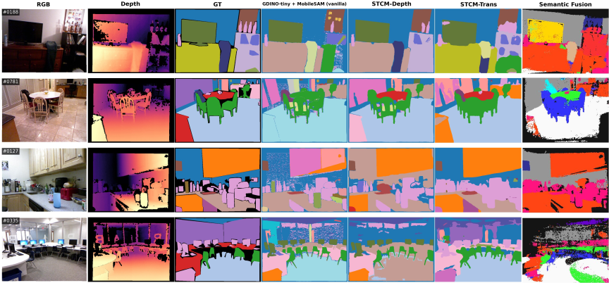
Fig. 8. Qualitative comparison on four NYUv2 test scenes. Columns (left \(\to\) right): RGB input, Kinect depth, NYUv2-40 ground truth, vanilla GroundingDINO+MobileSAM zero-shot baseline, STCM-Depth (ours, training-free, depth variant), STCM-Trans (ours, supervised), and SemanticFusion (reference, NYUv2-13 class space).
Figure 8 shows side-by-side predictions on four representative NYUv2 test scenes (a living room, a dining area, an office room, and a classroom). Two patterns are visible. The gain from STCM-Depth over the vanilla baseline is concentrated on geometrically structured classes: floors and walls are recovered as coherent regions rather than fragmented patches, and the gravity-aligned plane prior largely resolves the floor-versus-ceiling confusion that dominates the vanilla column. The residual gap between STCM-Depth and the supervised STCM-Trans column is concentrated on cluttered small objects and NYU-40 catch-all classes, consistent with the open-vocabulary detector’s recall ceiling on cluttered scenes. SemanticFusion, included as a semantic-mapping reference rather than a like-for-like baseline, operates on a different (NYUv2-13) class space and so produces visibly coarser label boundaries.
5.6. Computational Performance and Static-Graph Deployment Feasibility
Hardware configuration is as follows: Intel Xeon w7-3465X CPU; NVIDIA RTX 6000 GPU; ROS 2 Humble, CUDA 12.4, PyTorch 2.4.0. Per-module latency aggregated over three rosbag replays is reported in Table 9. Mean, median (p50), and 95th-percentile (p95) latencies are given per module, alongside the effective per-bag rate (Eff. Hz, defined as the number of successful module updates divided by the bag duration). The analysis distinguishes the navigation-critical loop (FAST-LIO2 odometry, detection filter, LiDAR–image association, the place-GNG and instance-GNG updaters) whose profiled latency is small relative to the navigation update budget on the workstation, from asynchronous modules (GroundingDINO, MobileSAM, temporal fusion, end-to-end per-frame pipeline) that update at lower rates without blocking navigation. The LLM grounder is not in the per-frame timing budget: it is invoked once per user command with decoding temperature set to \(0\) rather than once per perception frame, so its latency is amortized over a navigation episode rather than over a sensor cycle.
| Module | Class | Mean [ms] | p50 [ms] | p95 [ms] | Eff. Hz |
| FAST-LIO2 odom (publish) | critical | — | — | — | \(7.7\) |
| GroundingDINO detect\(^{‡}\) | async | \(164\) | \(157\) | \(162\) | \(0.9\) |
| MobileSAM segment | async | \(62.9\) | \(62.5\) | \(70.3\) | \(0.7\) |
| Detection filter | critical | \(0.2\) | \(0.2\) | \(0.3\) | \(0.9\) |
| LiDAR–image assoc\(^{†}\) | critical | \(4.3\) | \(1.4\) | \(13.2\) | \(1.5\) |
| Instance-GNG update | critical | \(9.0\) | \(11.1\) | \(22.5\) | \(1.3\) |
| Place-GNG update | critical | \(17.3\) | \(21.5\) | \(22.1\) | \(0.9\) |
| Temporal fusion | async | \(39.4\) | \(30.7\) | \(87.4\) | \(0.7\) |
| Per-frame pipeline | async | \(1693\) | \(1969\) | \(2468\) | \(0.9\) |
Summing critical-path p95 latencies of the STCM-side modules at the operating point used for evaluation (detection filter, LiDAR–image association, instance-GNG, place-GNG) yields approximately \(58\) ms per detection cycle. This is the per-cycle latency of the STCM update kernels when an input observation is available; it is distinct from the actual rate at which those kernels are invoked, which is determined by the slower upstream semantic modules. FAST-LIO2 publishes its odometry topic at \(7.7\) Hz, well within the open-loop latency the place-graph update can absorb (\(\sim 22\) ms p95). The STCM update kernels could therefore service input at rates well above the navigation update budget if observations arrived faster, but in practice the per-frame semantic stream arrives at roughly \(0.7\)–\(1.5\) Hz on this workstation, so end-to-end graph updates occur at module-rate rather than at low-latency limit. Obstacle avoidance remains served by FAST-LIO2 and the LiDAR costmap at \(7.7\) Hz, decoupled from the slower semantic update. The slowest single module (GroundingDINO at \(164\) ms mean / \(162\) ms p95) is asynchronous and does not block Nav2; the practical consequence is a semantic-update lag of order one second between an object entering the camera view and its node being committed. This supports operation in stationary or slow-moving assistive settings.
The workstation-class budget reported above pertains to the map-building stage of STCM, which is a one-shot offline procedure rather than a recurring online cost. In the intended deployment model, the foundation-model-heavy perception components (GroundingDINO, MobileSAM) and the dual-GNG learner are executed once on a high-compute workstation during an initial mapping pass (or rosbag replay) through the environment. The resulting place graph, instance set, and accumulated semantic scores are serialized to the stcm.json artifact described in Subsection 5.7. At robot run-time, the on-board computer (e.g., an NVIDIA Jetson on the Ranger Garden Assistant platform used here) consumes this JSON as a static knowledge layer: localization is provided by the localization mode of our FAST-LIO2 ROS 2 stack, which relocalizes against the point-cloud map saved during the mapping pass (built in the same stack’s SLAM mode), so the runtime pose is published in the same map frame as the serialized stcm.json, and navigation is carried out by Nav2 using waypoints retrieved from the JSON-encoded place graph. The LLM grounder is not part of the mapping pipeline; instead, it is invoked at command time on the serialized graph to map a natural-language request to a target node identifier, so it operates on a static knowledge layer rather than on per-frame perception. Re-running the open-vocabulary detection and graph-learning pipeline on the embedded device for creating a map is therefore not required for navigation.
5.7. Online Place Graph Construction
We demonstrate incremental STCM construction during a teleoperated mapping traversal of a separate corridor environment, distinct from the three S1–S3 evaluation bags reported in Table 3. The robot begins with an empty place graph and incrementally adds nodes as it explores. Fig. 9 shows a top-down 2D projection of the metric map \(\mathcal{M}\) generated online by FAST-LIO2 during a single traversal (approximately 5 minutes of operation). This metric layer provides the map-frame pose stream used by place-GNG to discretize the trajectory into revisitable places. The resulting STCM contains 54 place nodes, 65 place-to-place edges, and 24 anchored semantic object instances, capturing the corridor’s main structure: a dense sequence of places along the hallway with branches at doorways and the water fountain alcove.
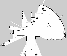
Fig. 9. Top-down 2D projection of the metric LiDAR map \(\mathcal{M}\) produced online by FAST-LIO2 during corridor mapping. The visualization provides the metric context in which STCM operates: the FAST-LIO2 pose stream defines the robot trajectory used by place-GNG to create a sparse place graph, while the metric map supports waypoint execution and collision-aware local planning.
Node spacing is approximately 0.5–0.8 m, consistent with the \(D_{\text{new}} = 0.5\) m threshold and local GNG adaptation. Edges reflect proximity relations, observed traversal relations, or both: the main corridor produces a chain structure, while areas where the robot turned around or looped (e.g., approaching the water fountain and returning) produce additional cross-connections.
5.8. Semantic Label Fusion and Stability
Semantic labels are accumulated into place nodes over repeated visits. Initially, nodes have no dominant label (uniform zero scores). As the robot observes objects near a place, the corresponding semantic scores increase. Table 10 shows example nodes with their accumulated semantic scores from the experimental corridor navigation run; the “Label” column reports the dominant class for each node (the \(\arg\max_c s_{i,c}\) assignment of Eq. (24)), which is not the same as the stability flag used in Table 11: a dominant label can be assigned at any positive score, while the LabelCov stability flag requires \(\max_c s_{i,c} > 0.55\). Several of the rows in Table 10 therefore expose dominant labels whose accumulated score is below the LabelCov threshold and would not be counted as stable for the purposes of Table 11. Representative semantic detection results for different place categories are shown in Fig. 10.
| Node | Visits | Semantic scores | Label |
| 0 | 49 | water fountain: 0.20 | water fountain |
| 14 | 27 | trash bins: 0.59, water fountain: 0.49, chair: 0.28 | trash bins |
| 22 | 30 | bottle: 0.26, trash bins: 0.10, cup: 0.08 | bottle |
| 35 | 18 | chair: 0.14, desk: 0.10 | chair |
| 11 | 11 | trash bins: 0.56, cardboard box: 0.38, water fountain: 0.35 | trash bins |
| Method | \(\boldsymbol{|P|}\) | LabelCov \(\boldsymbol{↑}\) | \(\boldsymbol{|S|}\) | \(\boldsymbol{|E_S|^{†}}\) | Mean stability \(\boldsymbol{↑}\) | \(\boldsymbol{|\Delta S|/|S_{GT}|↓}\) |
| Semantic-only | – | – | 197\(^{‡}\) | 2469 | – | 9.368 |
| Semantic + place-GNG (no instance GNG) | 59 | – | 28 | 56 | – | 0.474 |
| Dual-GNG STCM (proposed) | 54 | 0.796 | 24 | 2 | 1.000 | 0.263 |
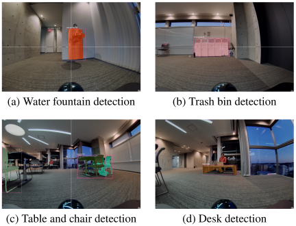
Fig. 10. Representative semantic detection results using GroundingDINO for open-vocabulary object detection in the corridor environment. Detections are temporally fused into STCM place nodes to create dominant semantic labels: (a) water fountain area, (b) trash bin area, (c) table/chair area, and (d) desk area.
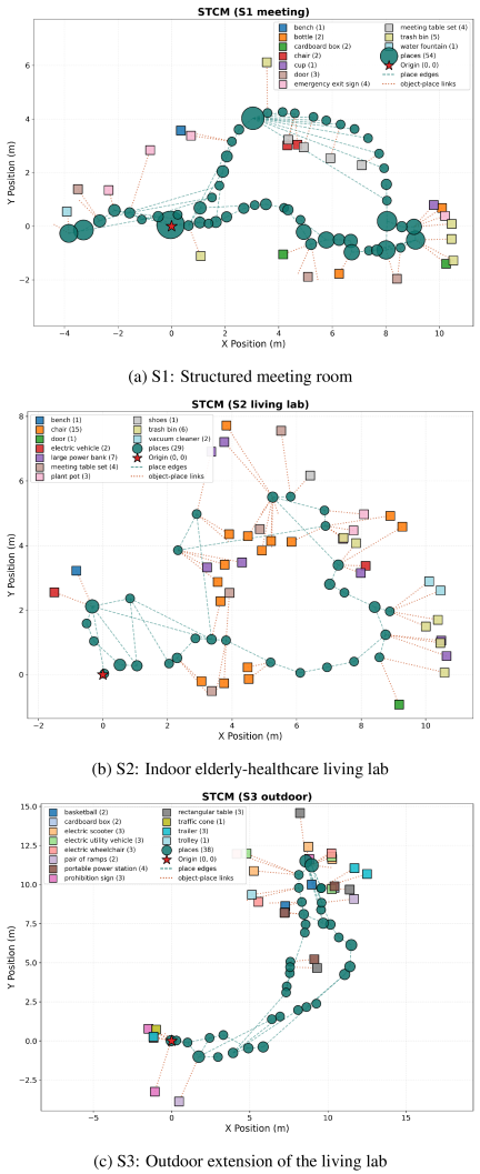
Fig. 11. STCM reconstructions plotted from the exported JSON graphs for the three evaluation scenes. Place nodes are circles in the map frame (marker size proportional to visit count); grounded object instances are shown at their anchored 2D positions, with edges depicting place-to-place connectivity and object–place associations. The same JSON serves as the structured representation queried by the LLM during deployment, enabling inspection of topological structure, semantic consistency, and graph serializability for downstream consumption.
Node labels stabilize over time despite frame-to-frame detection noise. For example, place node 0 near the water fountain area accumulates the highest visit count of the corridor run (49 visits) and a dominant water-fountain score of 0.20; the visit count, rather than the score itself, identifies it as the most frequently traversed landmark, and the score remains below the \(0.55\) LabelCov stability threshold defined in Section 5.7. Place node 14, visited 27 times, shows high scores for “trash bins” (0.59) along with co-occurring objects such as “water fountain” (0.49) and “chair” (0.28), reflecting the spatial proximity of these semantic features in the corridor. Place node 11 demonstrates multi-object accumulation, with scores for “trash bins” (0.56), “cardboard box” (0.38), and “water fountain” (0.35), indicating a location where multiple semantic objects are persistently detected across 11 visits.
The temporal fusion mechanism (\(\alpha = 0.1\)) filters detection errors. False positives from GroundingDINO (e.g., misclassifying a window reflection as a “bottle”) contribute low confidence and are outweighed by consistent detections of actual objects over multiple observations.
Figure 11 shows STCM reconstructions for the three evaluation scenes (S1, S2, S3), each plotted directly from the exported JSON graph in the map frame. Place nodes are drawn as circles whose marker size indicates the relative number of visits to each place; grounded object instances (GroundingDINO + SAM) are overlaid at their anchored 2D positions, and edges depict both place-to-place connectivity and object–place associations. The same JSON is the structured representation read by the LLM during deployment, so the visualization corresponds directly to the substrate consumed by graph search and language grounding (Section 3.8). Across the three scenes, the indoor structured meeting room (S1) and the indoor elderly-healthcare living lab (S2) produce compact place graphs over revisited regions, whereas the outdoor extension (S3) spans a longer trajectory with sparser place spacing and a reduced set of grounded indoor classes, reflecting the out-of-distribution vocabulary shift discussed in Section 5.1. The “meeting table set” target in S1 and S2 is a physical configuration consisting of a central table surrounded by two or four chairs, so chair instances are expected to cluster around the meeting-table anchor in the reconstruction rather than indicating spurious detections.
To quantitatively evaluate the contribution of each component in the STCM architecture, we compare the full dual-GNG STCM system against ablated variants. Table 11 reports key metrics across three configurations: a semantic-only approach that performs open-vocabulary detection without topological abstraction, a semantic mapping system augmented with place-GNG but without instance-level GNG fusion, and the proposed dual-GNG STCM with both place-level and instance-level GNG operating incrementally during the mapping pass. The metrics capture graph structure (\(|P|\) = number of place nodes) and object-level structure (\(|S|\) = number of persistent semantic object instances retained in the map after the mapping pass). LabelCov measures the fraction of place nodes with stable semantic labels, where a label is considered stable if its confidence score \(\max_c s_{i,c}\) exceeds 0.55 after sufficient observations. Mean stability quantifies instance position consistency by computing the standard deviation of instance centroid positions across revisits; instances with deviations below 0.15 m are deemed stable. The erroneous-detection count \(|E_S|\) tallies the number of raw detection events (i.e., per-frame observations) that the variant treats as evidence for an object but that do not correspond to any ground-truth object in the environment; it therefore counts spurious observations rather than persistent instances and can exceed \(|S|\) when many per-frame false detections collapse onto a few persistent prototypes (or, in the semantic-only baseline, fail to collapse at all because no temporal clustering is performed). Finally, semantic cardinality deviation \(|\Delta S|/|S_{GT}|\) measures the relative difference between the number of persistent detected instances and the ground-truth count \(|S_{GT}|\) for the corridor.
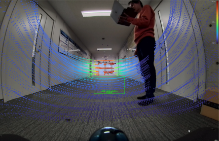
Fig. 12. Multi-modal fisheye-LiDAR sensor fusion. The 176° FOV fisheye camera captures wide-angle RGB imagery while the Livox Mid-360 provides dense 3D LiDAR point clouds. The system projects LiDAR points into the image frame (per-point \((u,v)\)) so that segmented detections can be associated directly with 3D LiDAR returns and then transformed to the map frame via TF, supporting consistent place labeling.
Table 11 suggests that the dual-GNG architecture is important for controlling duplicate instance creation: the semantic-only approach yields 197 raw detection-event prototypes accumulated by the open-vocabulary detector with 2469 erroneous detection events that do not correspond to any ground-truth object, producing a large semantic cardinality deviation (\(|\Delta S|/|S_{GT}|=9.368\)); this is consistent with the lack of spatial clustering, so per-frame false detections never collapse onto persistent instances under viewpoint variation and detection noise. Adding place-GNG without instance-GNG reduces over-segmentation (28 persistent instances, 56 erroneous detection events; \(|\Delta S|/|S_{GT}|=0.474\)) and yields a place graph (\(|P|=59\)), while place-level semantic coverage (LabelCov) is not reported for this ablation. In contrast, the proposed dual-GNG STCM reports \(|P|=54\) and achieves LabelCov of 0.796 with a mean stability of 1.000 (all instances below the 0.15 m position standard-deviation threshold across revisits), while reducing the persistent instance count to 24 with \(|E_S|=2\) erroneous detection events surviving fusion. Although the remaining cardinality deviation (0.263) indicates a residual mismatch in instance cardinality relative to the ground truth, these results indicate that combining place-level and instance-level GNG supports stable incremental semantic-topological mapping during the mapping pass in the evaluated setting.
5.9. Multi-Modal Sensor Fusion: Fisheye-LiDAR Integration
The wide-angle fisheye camera (176° FOV) provides substantially broader coverage than standard perspective cameras, enabling semantic detection of objects in peripheral regions that would otherwise require multiple viewpoints. LiDAR-camera fusion produces colorized point clouds that support both geometric mapping and semantic anchoring.
Figure 12 illustrates synchronized fisheye imagery and LiDAR point clouds. The fisheye lens captures the full corridor width and overhead structure in a single frame, while the Livox Mid-360’s non-repetitive scan accumulates dense 3D geometry. The system projects LiDAR points into the image frame and associates segmented detections (from GroundingDINO + SAM) with the subset of 3D points whose \((u,v)\) lie inside the mask, producing 3D-anchored semantic labels that are then transformed to the map frame via TF.
This multi-modal fusion improves robustness: the fisheye camera provides rich appearance cues for semantic classification, while LiDAR provides accurate metric positions unaffected by lighting variation or lens distortion. The combination enables reliable place labeling even in challenging conditions (e.g., backlit windows, shadowed corners).
5.10. Autonomous Navigation with STCM
We evaluate autonomous navigation using the constructed STCM graph. The robot is commanded to navigate to a place specified by semantic label (e.g., “go to the table area”). The system identifies the place node with the highest score for “table,” computes a graph path from the current node to the target node, and executes the path via Nav2 waypoint following.
Figure 13 shows a representative navigation trial. The robot successfully navigates from its starting position to the target place, following the topological path through intermediate nodes and using metric planning to avoid obstacles (e.g., a human crossing the corridor, a temporarily placed box). Nav2’s dynamic replanning handles local perturbations, while the topological graph provides stable waypoints that guide the global trajectory.
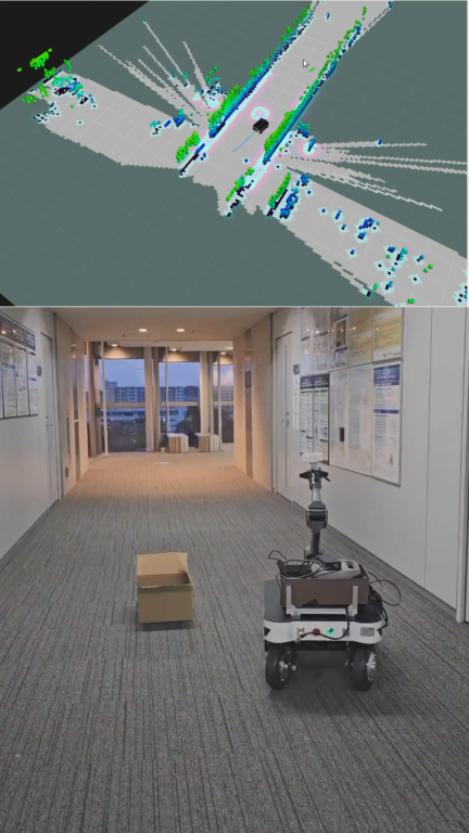
Fig. 13. Autonomous navigation with STCM. The robot navigates to a semantically specified goal (“go to the table area”) by planning over the STCM place graph and executing via ROS 2 Nav2 waypoint following. The topological graph provides stable high-level waypoints while Nav2 handles metric planning and local obstacle avoidance.
Across 10 navigation trials on the corridor demonstration described in Section 5.7 (separate from the S1–S3 offline graph-feasibility analysis of Section 5.2), the robot was issued semantic goals drawn from {table, water fountain, doorway, cardboard box} and achieved 9 successes and 1 failure. The single failure occurred when the target label “cardboard box” was ambiguous between two place nodes with similar accumulated scores for that label and the robot terminated at the incorrect node. Detailed per-trial start/goal poses, executed path lengths, durations, and per-trial success/failure criteria are not tabulated separately in this paper; the executed corridor trials are reported here as a complementary execution check on the offline graph-feasibility analysis of Section 5.2 rather than as the primary navigation benchmark.
5.11. Dynamic Human-as-Obstacle Avoidance
In assistive navigation scenarios, safe interaction with humans is critical. STCM does not include a dedicated human-detection module in the reported configuration: the Livox Mid-360 LiDAR returns 3D points from a human crossing the corridor and Nav2’s costmap layer treats those returns as dynamic obstacles, so the human is handled as a moving obstacle in the LiDAR costmap rather than as a classified “human” object. Nav2’s MPPI controller 32 then computes collision-free trajectories by optimizing sampled rollouts over this costmap. Fig. 14 shows the robot navigating around a human crossing its path. The costmap (constructed from LiDAR scans via the SpatioTemporalVoxelLayer) marks the human as an obstacle, and the MPPI controller generates a trajectory that slows and deviates laterally to maintain clearance while minimizing path deviation and control effort.
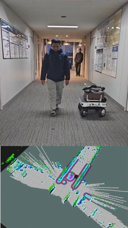
Fig. 14. Dynamic human-as-obstacle avoidance during STCM-guided navigation. The Livox Mid-360 LiDAR returns 3D points from the human in the corridor, which the Nav2 costmap layer treats as a moving obstacle (no dedicated human classifier is used), and Nav2’s MPPI controller computes a collision-free trajectory that maintains safe clearance. The STCM topological plan remains stable while metric planning handles the dynamic obstacle.
The STCM graph remains stable during such local perturbations: the robot’s high-level topological plan is unchanged, while metric planning handles dynamic obstacles.
5.12. Place Node Stability Analysis
To quantitatively assess the spatial distribution and coverage of semantic labels across the corridor environment, we analyze the position statistics of place nodes grouped by semantic label. Table 12 reports the number of place nodes with each label, total visit counts accumulated across all nodes of that label, and position standard deviations \(\sigma_x\) and \(\sigma_y\) that characterize the spatial extent of each semantic category.
| Semantic label | \(\boldsymbol{\sigma}_x\) [m] | \(\boldsymbol{\sigma}_y\) [m] | Nodes | Total visits | Avg. visits/node |
| Trash bins | 1.85 | 1.04 | 18 | 118 | 6.6 |
| Water fountain | 1.84 | 0.80 | 12 | 99 | 8.2 |
| Bottle | 0.00 | 0.00 | 1 | 30 | 30.0 |
| Chair | 1.81 | 2.07 | 4 | 21 | 5.2 |
| Cardboard box | 0.17 | 0.09 | 2 | 7 | 3.5 |
| Desk | 0.00 | 0.00 | 1 | 1 | 1.0 |
Note: \(\sigma\) is computed from the positions of all place nodes labeled with each semantic category. Single-node labels have \(\sigma = 0\) by definition.
Frequently occurring environmental features such as trash bins (18 nodes, 118 total visits) and water fountains (12 nodes, 99 total visits) appear across multiple place nodes throughout the corridor, with spatial extents \(\sigma_x \approx 1.8\) m and \(\sigma_y \approx 0.8\)–\(1.0\) m, reflecting the distribution of these place-node occurrences along the corridor topology; whether each occurrence corresponds to a physically distinct object instance or to repeated detections of the same object from different viewpoints is determined separately by the instance-level GNG and not by the row counts in Table 12. These values indicate that the STCM successfully captures the spatial spread of common corridor fixtures, enabling the robot to ground commands like “find a trash bin” to multiple candidate locations rather than a single fixed position.
The average visits per node metric quantifies the benefit of repeated traversals and temporal evidence accumulation. The single bottle node accumulated 30 visits, the highest per-node average, indicating that the robot repeatedly passed through this location and consistently reinforced the semantic label through temporal fusion. In contrast, water fountain and trash bin nodes show moderate per-node averages (8.2 and 6.6, respectively), as visits are distributed across multiple spatial instances of these categories. This difference reflects the underlying environment structure: unique objects accumulate all revisit evidence at one node, while distributed object categories spread evidence across their spatial instances.
Labels appearing at a single location (bottle, desk) exhibit \(\sigma \approx 0\) by definition, while labels appearing at multiple locations (chair, cardboard box, trash bins, water fountain) show non-zero standard deviations that characterize their spatial distribution. This distinction has important implications for navigation planning: localized labels serve as unique landmarks that provide unambiguous goal targets, while distributed labels require disambiguation through additional context (e.g., “go to the nearest trash bin” vs. “go to the trash bin near the water fountain”). Future work may incorporate spatial-relational reasoning to automatically resolve such ambiguities using the place graph topology.
6. Discussion
6.1. Design Rationale and Trade-Offs
The STCM architecture reflects a deliberate trade-off between representational richness and practical integration. Dense semantic mapping approaches (e.g., ConceptFusion, VLMaps) provide high-resolution spatial queries and fine-grained object-level reasoning, but often require substantial computational resources and may not directly interface with standard navigation stacks. Full scene graph systems (e.g., Hydra, S-Graphs+) support rich relational reasoning but emphasize global optimization and may not prioritize temporal fusion of open-vocabulary detections or lightweight goal grounding. A recent comparative evaluation of open-source topological mapping methods reports that current pipelines remain navigation-fragile in specific ways, including graph disconnection under noisy positioning and a non-trivial fraction of edges crossing obstacles 55, motivating compact, inspectable graph representations of the kind STCM provides.
STCM prioritizes interpretability, learnability, and ROS 2 compatibility. The place graph is sparse (tens of nodes rather than thousands of landmarks), enabling efficient graph search and transparent explanation of navigation decisions to users. Semantic labels are accumulated over time via simple exponential smoothing, avoiding the need for complex probabilistic inference or offline training. The graph is directly serializable and visualizable, supporting debugging and user inspection. This is conceptually aligned with the spatial semantic hierarchy 56, which describes spatial knowledge as a hierarchy in which a topological layer of places and connections sits between sensorimotor and metric levels and provides a symbolic layer over which routes can be reasoned about; STCM borrows this layered framing as a design heuristic rather than as a claim about cognitive realism or about human-style route explanation, which are not evaluated here.
From an ecological psychology perspective, behavior generation depends on how an individual’s perceptual systems detect affordances, which are actionable properties of the environment that support specific activities 5,2. In STCM, place nodes implicitly capture navigational affordances: a node labeled “doorway” affords passage between rooms, while a node labeled “table” affords approach for object manipulation. The multi-scopic organization separates concerns by temporal and spatial scale: microscopic processes detect immediate affordances (e.g., a suddenly obstructed foothold), mesoscopic processes accumulate affordances into place representations (e.g., recognizing that a location consistently affords visibility of the water fountain), and macroscopic processes reason about affordance sequences for goal achievement (e.g., planning a route through a series of navigable places). This separation enables efficient computational resource allocation: the system dedicates high-frequency, low-latency processing to immediate sensorimotor demands while deferring global reasoning to lower-frequency updates. This organization is consistent with the multi-scopic design view introduced as motivation, separating fast metric control from slower semantic and graph-level reasoning, and should be interpreted as an engineering abstraction rather than as a validated cognitive model 2. In the reported experiments it supports local adaptation through Nav2 replanning and efficient long-horizon planning over the place graph, rather than any formal notion of optimal navigation.
The choice of GNG for topological learning provides automatic node creation and topology adaptation without requiring manual place annotation or supervised training. The present experiments demonstrate incremental graph construction during a recorded mapping traversal and subsequent use of the serialized graph for navigation; the incremental nature of GNG is compatible with future lifelong map maintenance, but the current evaluation does not test long-term cross-session updating, loop-closure-aware graph repair, or persistent adaptation in changing homes. Multi-scale variants of GNG 26 can be integrated in future work to support hierarchical place abstractions (e.g., room-level and building-level graphs).
The use of GroundingDINO for open-vocabulary detection enables flexible semantic prompting without retraining. The graph interface is designed to allow goals to be specified through familiar references to task-relevant landmarks (“medicine cabinet,” “bedside table”) that may not appear in standard closed-set object-detection datasets, subject to detector recall and prompt sensitivity. MobileSAM refines detected boxes into masks in the reported configuration; its per-frame cost motivates future selective invocation strategies, such as conditioning on detector confidence or downstream disambiguation needs.
6.2. Semantic Grounding Challenges
Despite the promise of foundation models, semantic grounding remains challenging in real indoor environments. GroundingDINO detection quality varies with object appearance, occlusion, and prompt phrasing. Small or partially occluded objects (e.g., a cup on a table behind a chair) may be missed, while visually similar categories (e.g., “trash bin” vs. “cardboard box”) can be confused. Transparent and reflective surfaces (glass windows, polished floors) produce detection artifacts. As a large model, GroundingDINO requires significant computational resources and can still fail on unusual phrasing or abstract semantic queries 27. Similarly, while SAM provides powerful segmentation capabilities, it can over-segment or under-segment in complex scenes and was trained primarily on daily objects, potentially missing specialized indoor landmarks 28.
Figure 15 illustrates a representative failure mode where motion blur and challenging lighting conditions degrade open-vocabulary detection performance. Such failure cases highlight the importance of temporal fusion: single-frame errors are mitigated by accumulating evidence over multiple observations, but initial detection failures can delay or prevent place label assignment.
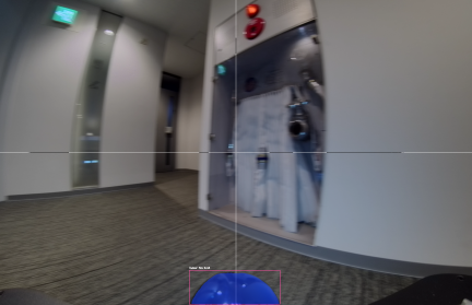
Fig. 15. Failure case in semantic grounding. Motion blur, occlusion, and challenging lighting conditions degrade GroundingDINO detection quality, resulting in missed or incorrect object labels. Temporal fusion mitigates single-frame errors but requires multiple observations to stabilize labels. Future work should incorporate more stable image capture and confidence-aware fusion strategies.
Temporal fusion into place nodes mitigates single-frame errors but introduces latency: a place label becomes stable only after multiple observations. In dynamic environments where objects move frequently, this may lead to stale labels. Future work could incorporate explicit object tracking and change detection to distinguish persistent place fixtures (e.g., a “water fountain” or a “doorway”) from transient objects (“cup on table”).
Range-based 3D grounding via image-projected LiDAR provides reliable metric anchors but introduces sparsity and calibration sensitivities. LiDAR beams may miss small or thin objects, and imperfect camera–LiDAR calibration can cause projected points to fall outside a segmentation mask. Robust association and outlier handling remain important; in particular, sparse returns can cause unstable 3D anchors for slender structures (e.g., chair legs). When needed, a dense monocular depth estimator (Depth Anything 44) can be used as an optional fallback for masks with no LiDAR hits, but it requires careful validation of scale and failure modes. Depth Anything provides relative depth predictions that must be scaled to metric units, typically via a scale factor estimated from LiDAR correspondences or prior calibration, and its accuracy degrades for distant objects or scenes with large depth discontinuities. The depth fallback mechanism was not employed in the experiments reported in this paper.
6.3. STCM for Assistive Human-Robot Interaction
STCM is motivated by assistive navigation in domestic and care environments, where users are often non-expert and goals are expressed through familiar places and objects rather than metric coordinates. Labels such as “kitchen,” “bedside,” and “near the medicine cabinet” refer to function and affordance as much as geometry.
Metric SLAM provides the foundation for safe motion, but it does not by itself support this symbolic, language-mediated form of reference. STCM addresses the gap by coupling the metric map with an explicit place graph carrying open-vocabulary semantic labels. The graph interface is designed to allow goals to be specified as familiar references rather than raw metric waypoints, and the system resolves these requests by selecting graph nodes whose semantic labels match the description; the evaluated command sets test this mechanism under controlled conditions rather than in unconstrained domestic use. Prior work has shown that semantic maps can support natural-language navigation instructions 57; STCM extends this idea by using open-vocabulary detection for configured or prompted task-relevant landmarks, such as potential references to a “medicine cabinet,” “favorite reading chair,” or “bedside table,” subject to perception recall and without task-specific detector retraining.
The representation is practical for a deployment model in which the semantic-topological graph is built during an initial mapping pass and then consumed as a static knowledge layer at runtime: place nodes, semantic-score vectors, object instances, and graph edges are stored in a serialized stcm.json artefact that can be inspected and visualized rather than hidden in latent feature fields, and the navigation-critical loop reads from this artefact while semantic updates remain asynchronous. This node-level structure is consistent with HRI evidence that robot self-explanations can improve how humans understand and evaluate robot behaviour 58, and with broader recent arguments that vision–language transparency mechanisms can contribute to trust in mobile-robot settings 59; this paper does not itself evaluate user-facing trust, explanation quality, or long-term assistive effectiveness.
6.4. Limitations and Future Directions
STCM should be interpreted as a deployment-oriented semantic-topological representation rather than as a replacement for dense open-vocabulary maps, full 3D scene graphs, or benchmark-specialized navigation systems. The present evidence supports map-frame semantic grounding, object-graph construction, functional-command grounding when relevant target labels are recoverable in the graph, non-blocking static-graph deployment on Nav2, and real-platform integration.
The current study therefore does not yet evaluate long-term assistive use, user-facing trust, or persistent operation across changing environments. The graph also inherits errors from the underlying SLAM system, and the current implementation does not explicitly separate static scene structure from movable objects. Consequently, map updates and object relocation can affect place-node positions, semantic anchors, and the stability of temporally fused labels.
Future work should therefore focus on explicit object tracking and change detection, loop-closure-aware graph maintenance, cross-session relocalization, broader navigation evaluation, and user studies in realistic home environments.
7. Conclusion
This paper presented STCM, a semantic-topological cognitive map constructed during an initial mapping pass and serialized as a reusable graph artefact for assistive indoor navigation. STCM connects FAST-LIO2 LiDAR-inertial localization, dual GNG graph construction during mapping, open-vocabulary semantic grounding, language-driven goal specification, and ROS 2/Nav2 execution on a real mobile robot. The pipeline is split between a workstation-side mapping phase, in which the foundation-model-heavy perception modules and the dual-GNG learner are run once to produce the serialized stcm.json, and a robot-side runtime phase, in which FAST-LIO2 localization and Nav2 consume the prebuilt graph as a static knowledge layer and the LLM is invoked once per user command to map natural language to a target node rather than once per perception frame. Its central contribution is a compact, serializable place graph in which revisitable locations, semantic object evidence, and navigation connectivity are grounded in the map frame and exposed through an explicit language-to-graph interface. The evaluation supports this deployment-oriented design. On NYUv2-40, the depth-only perception variant improves zero-shot mIoU from \(26.11\) to \(39.24\) over the GroundingDINO+MobileSAM baseline. Across three recorded scenes, the prompt-bank STCM backend obtains a macro-mean object-graph \(F_1\) of \(0.480\), compared with \(0.404\) for the strongest prior-augmented variant, with the S3 component obtained under post-hoc alias tuning and reported as a diagnostic probe.
The language-grounding ablation further indicates the benefit of explicit graph grounding, increasing meeting-scene functional-command accuracy from \(0.000\) to \(0.600\) (paired McNemar \(p = 0.0039\)). As a complementary execution check, a separate corridor demonstration produced nine successes in ten semantic-goal trials; the primary navigation metrics in this paper remain the offline graph-feasibility results of Section 5.2.
STCM is intentionally lighter than dense visual–language maps and less relationally expressive than full 3D scene graphs, but this trade-off enables direct coupling to an existing ROS 2/Nav2 stack and an inspectable stcm.json representation. The present study does not evaluate user-facing trust, long-term assistive effectiveness, dynamic object relocation, cross-session re-localization, or benchmark-aligned navigation against simulator-trained open-vocabulary navigation systems. Future work should address these gaps through more benchmark comparisons, user studies in realistic home environments, explicit object tracking and change detection, loop-closure-aware graph maintenance, and hierarchical multi-scale place graphs for larger buildings.
Acknowledgments
This work was supported by Japan Science and Technology Agency (JST), Moonshot R&D, with Grant Number JPMJMS2034.
- [1] P. A. Hancock, D. R. Billings, K. E. Schaefer, J. Y. C. Chen, E. J. de Visser, and R. Parasuraman, “A Meta-Analysis of Factors Affecting Trust in Human-Robot Interaction,” Human Factors, Vol.53, No.5, pp. 517-527, 2011. https://doi.org/10.1177/0018720811417254
- [2] A. A. Saputra, K. Wada, S. Masuda, and N. Kubota, “Multi-scopic Neuro-cognitive Adaptation for Legged Locomotion Robots,” Scientific Reports, Vol.12, Article No.16222, 2022. https://doi.org/10.1038/s41598-022-19599-2
- [3] E. C. Tolman, “Cognitive Maps in Rats and Men,” Psychological Review, Vol.55, No.4, pp. 189-208, 1948. https://doi.org/10.1037/h0061626
- [4] J. O’Keefe and L. Nadel, “The Hippocampus as a Cognitive Map,” Clarendon Press, 1978.
- [5] J. J. Gibson, “The Ecological Approach to Visual Perception,” Houghton Mifflin, 1979.
- [6] J. Woo and N. Kubota, “Recognition of Indoor Environment by Robot Partner Using Conversation,” J. Adv. Comput. Intell. Intell. Inform., Vol.17, No.5, pp. 753-760, 2013. https://doi.org/10.20965/jaciii.2013.p0753
- [7] N. Kubota and A. Yorita, “Topological Environment Reconstruction in Informationally Structured Space for Pocket Robot Partners,” Proc. IEEE Int. Symp. on Computational Intelligence in Robotics and Automation (CIRA), pp. 165-170, 2009. https://doi.org/10.1109/CIRA.2009.5423215
- [8] A. Rosinol, M. Abate, Y. Chang, and L. Carlone, “Kimera: An Open-Source Library for Real-Time Metric-Semantic Localization and Mapping,” Proc. IEEE Int. Conf. on Robotics and Automation (ICRA), 2020. https://doi.org/10.1109/ICRA40945.2020.9196885
- [9] N. Hughes, Y. Chang, and L. Carlone, “Hydra: A Real-time Spatial Perception System for 3D Scene Graph Construction and Optimization,” Proc. Robotics: Science and Systems (RSS), 2022. https://doi.org/10.15607/RSS.2022.XVIII.050
- [10] H. Bavle, J. L. Sánchez-López, M. Shaheer, J. Civera, and H. Voos, “S-Graphs+: Real-Time Localization and Mapping Leveraging Hierarchical Representations,” IEEE Robotics and Automation Letters, Vol.8, No.8, pp. 4927-4934, 2023. https://doi.org/10.1109/LRA.2023.3290512
- [11] C. Huang, O. Mees, A. Zeng, and W. Burgard, “Visual Language Maps for Robot Navigation,” Proc. IEEE Int. Conf. on Robotics and Automation (ICRA), pp. 10608-10615, 2023. https://doi.org/10.1109/ICRA48891.2023.10160969
- [12] K. M. Jatavallabhula, A. Kuwajerwala, Q. Gu, M. Omama, T. Chen, A. Maalouf, S. Li et al., “ConceptFusion: Open-Set Multimodal 3D Mapping,” Proc. Robotics: Science and Systems (RSS), 2023. https://doi.org/10.15607/RSS.2023.XIX.066
- [13] Q. Gu, A. Kuwajerwala, S. Morin, K. M. Jatavallabhula, B. Sen, A. Agarwal et al. “ConceptGraphs: Open-Vocabulary 3D Scene Graphs for Perception and Planning,” Proc. IEEE Int. Conf. on Robotics and Automation (ICRA), pp. 5021-5028, 2024. https://doi.org/10.1109/ICRA57147.2024.10610243
- [14] F. L. Busch, T. Homberger, J. Ortega-Peimbert, Q. Yang, and O. Andersson, “One Map to Find Them All: Real-Time Open-Vocabulary Mapping for Zero-Shot Multi-Object Navigation,” arXiv preprint, arXiv:2409.11764, 2024. https://doi.org/10.48550/arXiv.2409.11764
- [15] B. Chen, F. Xia, B. Ichter, K. Rao, K. Gopalakrishnan, M. S. Ryoo, A. Stone, and D. Kappler, “Open-Vocabulary Queryable Scene Representations for Real World Planning,” Proc. IEEE Int. Conf. on Robotics and Automation (ICRA), pp. 11509-11522, 2023. https://doi.org/10.1109/ICRA48891.2023.10161534
- [16] D. Shah, B. Osiński, B. Ichter, and S. Levine, “LM-Nav: Robotic Navigation with Large Pre-Trained Models of Language, Vision, and Action,” Proc. 6th Conf. on Robot Learning (CoRL), PMLR, Vol.205, pp. 492-504, 2022.
- [17] M. Chang, T. Gervet, M. Khanna, S. Yenamandra, D. Shah, S. Y. Min, K. Shah, C. Paxton, S. Gupta, D. Batra, R. Mottaghi, J. Malik, and D. S. Chaplot, “GOAT: GO to Any Thing,” Proc. Robotics: Science and Systems (RSS), 2024. https://doi.org/10.15607/RSS.2024.XX.073
- [18] Y. Tang, M. Wang, Y. Deng et al., “OpenIN: Open-Vocabulary Instance-Oriented Navigation in Dynamic Domestic Environments,” IEEE Robotics and Automation Letters, Vol.10, No.9, pp. 9256-9263, 2025. https://doi.org/10.1109/LRA.2025.3592071
- [19] S. Raychaudhuri, D. Ta, K. Ashton, A. X. Chang, J. Wang, and B. Bucher, “Zero-Shot Object-Centric Instruction Following: Integrating Foundation Models with Traditional Navigation,” arXiv preprint, arXiv:2411.07848, 2024. https://doi.org/10.48550/arXiv.2411.07848
- [20] L. Zhang, X. Hao, Q. Xu et al., “MapNav: A Novel Memory Representation via Annotated Semantic Maps for VLM-based Vision-and-Language Navigation,” Proc. 63rd Annual Meeting of the Association for Computational Linguistics (ACL), pp. 13032-13056, 2025. https://doi.org/10.18653/v1/2025.acl-long.638
- [21] D. S. Chaplot et al., “Neural Topological SLAM for Visual Navigation,” Proc. IEEE/CVF Conf. on Computer Vision and Pattern Recognition (CVPR), 2020. https://doi.org/10.1109/CVPR42600.2020.01289
- [22] D. An, H. Wang, W. Wang, Z. Wang, Y. Huang, K. He, and L. Wang, “ETPNav: Evolving Topological Planning for Vision-Language Navigation in Continuous Environments,” IEEE Trans. Pattern Anal. Mach. Intell., Vol.47, No.7, pp. 5130-5145, 2025. https://doi.org/10.1109/TPAMI.2024.3386695
- [23] S. Garg, K. Rana, M. Hosseinzadeh, L. Mares, N. Sünderhauf, F. Dayoub, and I. Reid, “RoboHop: Segment-Based Topological Map Representation for Open-World Visual Navigation,” Proc. IEEE Int. Conf. on Robotics and Automation (ICRA), pp. 4090-4097, 2024. https://doi.org/10.1109/ICRA57147.2024.10610234
- [24] W. Xu, Y. Cai, D. He, J. Lin, and F. Zhang, “FAST-LIO2: Fast Direct LiDAR-Inertial Odometry,” IEEE Trans. Robotics, Vol.38, No.4, pp. 2053-2073, 2022. https://doi.org/10.1109/TRO.2022.3141876
- [25] B. Fritzke, “A Growing Neural Gas Network Learns Topologies,” Advances in Neural Information Processing Systems (NeurIPS), Vol.7, pp. 625-632, 1994.
- [26] F. Ardilla, A. A. Saputra, and N. Kubota, “Multi-Scale Batch-Learning Growing Neural Gas Efficiently for Dynamic Data Distributions,” Int. J. Automation Technol., Vol.17, No.3, pp. 206-216, 2023. https://doi.org/10.20965/ijat.2023.p0206
- [27] S. Liu, Z. Zeng, T. Ren, F. Li, H. Zhang, J. Yang, Q. Jiang, C. Li, J. Yang, H. Su, J. Zhu, and L. Zhang, “Grounding DINO: Marrying DINO with Grounded Pre-Training for Open-Set Object Detection,” Proc. European Conf. on Computer Vision (ECCV), pp. 38-55, 2024. https://doi.org/10.1007/978-3-031-72970-6_3
- [28] A. Kirillov, E. Mintun, N. Ravi, H. Mao, C. Rolland, L. Gustafson, T. Xiao, S. Whitehead, A. C. Berg, W.-Y. Lo, P. Dollár, and R. Girshick, “Segment Anything,” Proc. IEEE/CVF Int. Conf. on Computer Vision (ICCV), pp. 3992-4003, 2023. https://doi.org/10.1109/ICCV51070.2023.00371
- [29] C. Zhang, D. Han, Y. Qiao, J. U. Kim, S.-H. Bae, S. Lee, and C. S. Hong, “Faster Segment Anything: Towards Lightweight SAM for Mobile Applications,” arXiv preprint, arXiv:2306.14289, 2023. https://doi.org/10.48550/arXiv.2306.14289
- [30] M. Ahn, A. Brohan, N. Brown, Y. Chebotar, O. Cortes, B. David, C. Finn et al., “Do As I Can, Not As I Say: Grounding Language in Robotic Affordances,” Proc. 6th Conf. on Robot Learning (CoRL), PMLR, Vol.205, pp. 287-318, 2022.
- [31] H. Zhang, H. Deng, J. Ou, and C. Feng, “Mitigating Spatial Hallucination in Large Language Models for Path Planning via Prompt Engineering,” Sci. Rep., Vol.15, Article No.8881, 2025. https://doi.org/10.1038/s41598-025-93601-5
- [32] S. Macenski et al., “The Marathon 2: A Navigation System,” Proc. IEEE/RSJ Int. Conf. on Intelligent Robots and Systems (IROS), 2020. https://doi.org/10.1109/IROS45743.2020.9341207
- [33] I. Armeni, Z.-Y. He, A. Zamir, J. Gwak, J. Malik, M. Fischer, and S. Savarese, “3D Scene Graph: A Structure for Unified Semantics, 3D Space, and Camera,” Proc. IEEE Int. Conf. on Computer Vision (ICCV), pp. 5664-5673, 2019. https://doi.org/10.1109/ICCV.2019.00576
- [34] U.-H. Kim, J.-M. Park, T.-J. Song, and J.-H. Kim, “3-D Scene Graph: A Sparse and Semantic Representation of Physical Environments for Intelligent Agents,” IEEE Trans. Cybern., Vol.50, No.12, pp. 4921-4933, 2020. https://doi.org/10.1109/TCYB.2019.2931042
- [35] Y. Tian, Y. Chang, F. H. Arias, C. Nieto-Granda, J. P. How, and L. Carlone, “Kimera-Multi: Robust, Distributed, Dense Metric-Semantic SLAM for Multi-Robot Systems,” IEEE Trans. on Robotics, Vol.38, No.4, pp. 2022-2038, 2022. https://doi.org/10.1109/TRO.2021.3137751
- [36] S. H. Allu, I. Kadosh, T. Summers, and Y. Xiang, “A Modular Robotic System for Autonomous Exploration and Semantic Updating in Large-Scale Indoor Environments,” arXiv preprint, arXiv:2409.15493, 2024. https://doi.org/10.48550/arXiv.2409.15493
- [37] N. Yokoyama, S. Ha, D. Batra, J. Wang, and B. Bucher, “VLFM: Vision-Language Frontier Maps for Zero-Shot Semantic Navigation,” Proc. IEEE Int. Conf. on Robotics and Automation (ICRA), pp. 42-48, 2024. https://doi.org/10.1109/ICRA57147.2024.10610712
- [38] D. S. Chaplot, D. Gandhi, A. Gupta, and R. Salakhutdinov, “Object Goal Navigation Using Goal-Oriented Semantic Exploration,” Advances in Neural Information Processing Systems (NeurIPS), 2020.
- [39] N. Zantout, H. Zhang, P. Kachana, J. Qiu, G. Chen, J. Zhang, and W. Wang, “SORT3D: Spatial Object-Centric Reasoning Toolbox for Zero-Shot 3D Grounding Using Large Language Models,” Proc. IEEE/RSJ Int. Conf. on Intelligent Robots and Systems (IROS), pp. 2201-2208, 2025. https://doi.org/10.1109/IROS60139.2025.11246145
- [40] X. Huang, S. Zhao, Y. Wang et al., “MSGNav: Unleashing the Power of Multi-modal 3D Scene Graph for Zero-Shot Embodied Navigation,” arXiv preprint, arXiv:2511.10376, 2025. https://doi.org/10.48550/arXiv.2511.10376
- [41] H. Zhou, X. Wang, H. Li et al., “LagMemo: Language 3D Gaussian Splatting Memory for Multi-modal Open-Vocabulary Multi-Goal Visual Navigation,” arXiv preprint, arXiv:2510.24118, 2025. https://doi.org/10.48550/arXiv.2510.24118
- [42] J. Crespo, J. C. Castillo, O. M. Mozos et al., “Semantic Information for Robot Navigation: A Survey,” Applied Sciences, Vol.10, No.2, Article No.497, 2020. https://doi.org/10.3390/app10020497
- [43] R. Alqobali, M. Alshmrani, R. Alnasser et al., “A Survey on Robot Semantic Navigation Systems for Indoor Environments,” Applied Sciences, Vol.14, No.1, Article No.89, 2024. https://doi.org/10.3390/app14010089
- [44] L. Yang, B. Kang, Z. Huang, X. Xu, J. Feng, and H. Zhao, “Depth Anything: Unleashing the Power of Large-Scale Unlabeled Data,” Proc. IEEE/CVF Conf. on Computer Vision and Pattern Recognition (CVPR), pp. 10371-10381, 2024. https://doi.org/10.1109/CVPR52733.2024.00987
- [45] A. Junaedy, H. Masuta, Y. Fuse, K. Sawai, T. Motoyoshi, and N. Takagi, “Online Topological Mapping on a Quadcopter with Fast Growing Neural Gas,” J. Adv. Comput. Intell. Intell. Inform., Vol.28, No.6, pp. 1354-1366, 2024. https://doi.org/10.20965/jaciii.2024.p1354
- [46] A. Radford, J. W. Kim, C. Hallacy, A. Ramesh, G. Goh, S. Agarwal, G. Sastry, A. Askell, P. Mishkin, J. Clark, G. Krueger, and I. Sutskever, “Learning Transferable Visual Models from Natural Language Supervision,” Proc. Int. Conf. on Machine Learning (ICML), PMLR, Vol.139, pp. 8748-8763, 2021.
- [47] J. Long, E. Shelhamer, and T. Darrell, “Fully Convolutional Networks for Semantic Segmentation,” Proc. IEEE Conf. on Computer Vision and Pattern Recognition (CVPR), pp. 3431-3440, 2015. https://doi.org/10.1109/cvpr.2015.7298965
- [48] D. Eigen and R. Fergus, “Predicting Depth, Surface Normals and Semantic Labels with a Common Multi-Scale Convolutional Architecture,” Proc. IEEE Int. Conf. on Computer Vision (ICCV), pp. 2650-2658, 2015. https://doi.org/10.1109/iccv.2015.304
- [49] C. Hazirbas, L. Ma, C. Domokos, and D. Cremers, “FuseNet: Incorporating Depth into Semantic Segmentation via Fusion-based CNN Architecture,” Asian Conf. on Computer Vision (ACCV), pp. 213-228, 2016. https://doi.org/10.1007/978-3-319-54181-5_14
- [50] S. Lee, S.-J. Park, and K.-S. Hong, “RDFNet: RGB-D Multi-level Residual Feature Fusion for Indoor Semantic Segmentation,” Proc. IEEE Int. Conf. on Computer Vision (ICCV), pp. 4990-4999, 2017. https://doi.org/10.1109/iccv.2017.533
- [51] J. McCormac, A. Handa, A. Davison, and S. Leutenegger, “SemanticFusion: Dense 3D Semantic Mapping with Convolutional Neural Networks,” Proc. IEEE Int. Conf. on Robotics and Automation (ICRA), pp. 4628-4635, 2017. https://doi.org/10.1109/icra.2017.7989538
- [52] X. Hu, K. Yang, L. Fei, and K. Wang, “ACNet: Attention Based Network to Exploit Complementary Features for RGBD Semantic Segmentation,” Proc. IEEE Int. Conf. on Image Processing (ICIP), pp. 1440-1444, 2019. https://doi.org/10.1109/icip.2019.8803025
- [53] X. Chen, K.-Y. Lin, J. Wang, W. Wu, C. Qian, H. Li, and G. Zeng, “Bi-directional Cross-Modality Feature Propagation with Separation-and-Aggregation Gate for RGB-D Semantic Segmentation,” European Conf. on Computer Vision (ECCV), pp. 561-577, 2020. https://doi.org/10.1007/978-3-030-58621-8_33
- [54] D. Seichter, M. Köhler, B. Lewandowski, T. Wengefeld, and H.-M. Gross, “Efficient RGB-D Semantic Segmentation for Indoor Scene Analysis,” Proc. IEEE Int. Conf. on Robotics and Automation (ICRA), pp. 13525-13531, 2021. https://doi.org/10.1109/ICRA48506.2021.9561675
- [55] K. Muravyev and K. Yakovlev, “Evaluation of Topological Mapping Methods in Indoor Environments,” IEEE Access, Vol.11, pp. 132683-132698, 2023. https://doi.org/10.1109/ACCESS.2023.3335818
- [56] B. Kuipers, “The Spatial Semantic Hierarchy,” Artif. Intell., Vol.119, Nos.1-2, pp. 191-233, 2000. https://doi.org/10.1016/S0004-3702(00)00017-5
- [57] S. Tellex, T. Kollar, S. Dickerson, M. Walter, A. Banerjee, S. Teller, and N. Roy, “Understanding Natural Language Commands for Robotic Navigation and Mobile Manipulation,” Proc. AAAI Conf. on Artificial Intelligence, pp. 1507-1514, 2011. https://doi.org/10.1609/aaai.v25i1.7979
- [58] S. Stange and S. Kopp, “Effects of a Social Robot’s Self-Explanations on How Humans Understand and Evaluate Its Behavior,” Proc. ACM/IEEE Int. Conf. on Human-Robot Interaction (HRI), pp. 619-627, 2020. https://doi.org/10.1145/3319502.3374802
- [59] O. Sotomi, D. Kodi, and A. Arab, “Trust Through Transparency: Explainable Social Navigation for Autonomous Mobile Robots via Vision-Language Models,” arXiv preprint, arXiv:2504.05477, 2025. https://doi.org/10.48550/arXiv.2504.05477
Appendix
Appendix A. Abbreviations
Abbreviations used in this paper are presented in Table 13.
| Abbreviation | Expansion |
| SLAM | Simultaneous localization and mapping |
| LLM | Large language model |
| STCM | Semantic-topological cognitive map |
| GNG | Growing neural gas |
| LiDAR | Light detection and ranging |
| LIO | LiDAR–inertial odometry |
| ROS 2 | Robot Operating System 2 |
| Nav2 | Navigation2 |
| SAM | Segment Anything model |
| FAST-LIO2 | Fast direct LiDAR-inertial odometry 2 |
| NYUv2 | New York University Depth Dataset v2 |
| CLIP | Contrastive language-image pretraining |
| IMU | Inertial measurement unit |
| RGB-D | Red–green–blue plus depth |
| mIoU | Mean intersection over union |
| pAcc | Pixel accuracy |
| mAcc | Mean class accuracy |
| GT | Ground truth |
| GDINO | GroundingDINO (used only in space-constrained |
| figure/table labels) | |
| COCO | Common objects in context |
| AP | Average precision |
| ViT | Vision Transformer |
This article is published under a Creative Commons Attribution-NoDerivatives 4.0 Internationa License.