
Research Paper:
Anomaly Detection in Time Series with Enhanced Privacy Using Self-Supervised Contrastive Learning
Chihiro Maru*,†
 , Masato Oguchi**
, Miyuki Nakano***, and Ichiro Kobayashi**
*Faculty of Science and Engineering, Chuo University
1-13-27 Kasuga, Bunkyo-ku, Tokyo 112-8551, Japan
†Corresponding author
**Graduate School of Humanities and Sciences, Ochanomizu University
2-1-1 Otsuka, Bunkyo-ku, Tokyo 112-8610, Japan
***College of Liberal Arts, Tsuda University
2-1-1 Tsuda-machi, Kodaira, Tokyo 187-8577, Japan

Anomaly detection in time series is increasingly used for sensitive data, including medical and physiological data. However, these data carry a substantial risk of information leakage, making privacy preservation through anonymization essential. While anonymization reduces the risk of privacy breach, it can also remove informative features, creating a trade-off between privacy preservation and anomaly-detection performance. To address this challenge, we propose a robust framework that mitigates this trade-off and enables high-accuracy anomaly detection on anonymized data. Our approach centers on an anonymization function that transforms a time series by removing sensitive information, including contextual features and personally identifiable information, while retaining information that is beneficial for anomaly detection. We introduced a privacy model that guides the training of the anonymization function and optimizes the two components in an adversarial manner using contrastive loss in opposite directions. This design uses the anonymization function to eliminate sensitive information captured by the privacy model. We incorporate an anomaly detection loss function to ensure that the anonymization function preserves the essential information required for accurate anomaly detection. The effectiveness of the anonymization process and its impact on anomaly-detection performance were evaluated using multiple real-world and synthetic datasets. Results showed that our method reduced privacy-related information leakage by 42.65% while incurring only a 2.58% decrease in the F1 score for anomaly detection.
Privacy-enhanced anomaly detection framework
1. Introduction
Advancements in Anomaly Detection. The development of information and communication technology has enabled the real-time collection of vast amounts of data across various domains. Analytical technologies capable of handling such large data, such as machine learning and deep learning, have significantly advanced. A prominent application of these data-analysis technologies is time-series anomaly detection, which has performed highly in diverse fields, including healthcare, smart cities, and finance 1,2,3. An anomaly, in the context of anomaly detection, is a data point or a sequence of data points that deviates from normal behavior. Examples include outliers and noise in natural phenomena, fraud and human error in human activities, and measurement deviations and malfunctions in system operations. Detecting these anomalies with high precision can enhance safety and reduce operational costs, making anomaly detection critical in numerous real-world applications.
Anomaly Detection for Sensitive Data. Anomaly detection is vital in safety-critical domains, such as home security systems (detecting intrusions and abnormal activities), patient monitoring (identifying medical emergencies), and detection of cyberattacks and failures in critical infrastructure 4. These domains frequently handle data with high confidentiality requirements, making them constant targets for data theft or misuse by malicious actors 5,6. To protect the privacy of such sensitive information, anonymization is necessary to ensure that the content of the data remains indecipherable even if leaks occur 4,7,8.
Anonymization of Time Series. In this study, we define the anonymization of time series as a combined process of removing personally identifiable information (PII) and eliminating contextual features inherent to the time series.
Data anonymization generally involves the removal of PII, such as names, ages, and social security numbers, to prevent the identification of specific individuals or attributes 9. This concept is also applicable to time-series data, where the appropriate removal of PII is crucial, where such information is present 10,11. Recently, research on applying time-series analysis to large language models, as well as developing foundational models for time series, has progressed rapidly 12,13,14. These models demonstrate high performance in various time-series analytical tasks. However, concerns have been raised regarding the potential use of PII contained within the training data for these models 15. Furthermore, leaks of PII included in training data owing to vulnerability have been reported 16.
Moreover, with the increasing prevalence of internet-of-things devices, lifestyle logs and health data are being used more frequently. Even when such data do not contain explicit PII, the contextual features of the time series can be used to infer personal behaviors and lifestyle patterns, posing significant privacy risks 4. For instance, analyzing electricity usage data can reveal the absence of the resident from home. This highlights that even time-series data without directly identifiable PII can raise privacy concerns owing to their inherent contextual features.
Limitations of Previous Studies. Research on data anonymization has primarily focused on encryption techniques and, more recently, machine-learning-based methods to eliminate contextual features of time-series data. Noise is often added to data to satisfy a privacy preservation metric known as differential privacy (DP) 17, which allows for anomaly detection using anonymized data. However, DP was not originally designed for time-series data, and simply adding noise does not always guarantee sufficient privacy preservation. For example, although anonymization may alter individual data points, the overall contextual features of the time-series data might still be discernible. Increasing the noise level to eliminate these contextual features could mitigate this risk; however, it may significantly degrade data quality, rendering it less useful for downstream tasks. This is particularly problematic as these anonymization methods are typically developed without considering downstream tasks such as anomaly detection. Consequently, using such anonymized data can degrade anomaly-detection accuracy.
Challenges Addressed in This Study. A fundamental trade-off exists between achieving sufficient privacy preservation and maintaining high anomaly-detection performance; however, both objectives are critical and should ideally be compatible 4. To address this challenge, we develop a framework that facilitates anomaly detection on anonymized time-series data while achieving accuracy comparable to that with non-anonymized data. Within this framework, we define time-series data anonymization as the removal of both PII and contextual features. Based on this definition, we designed an anonymization function that eliminates sensitive information while retaining the features essential for accurate anomaly detection. We trained this anonymization function using a combined loss function that incorporates both contrastive learning and anomaly detection losses. Furthermore, we incorporated adversarial training to ensure the removal of PII and contextual features. This approach allows the preservation of privacy while maintaining the data utility for anomaly-detection tasks. To the best of our knowledge, this is the first study to combine data security through anonymization with task performance in anomaly detection. The contributions of this study can be summarized as follows:
-
・
We developed a framework that balances the trade-off between privacy preservation and anomaly-detection accuracy, ensuring sufficient performance for practical applications even with anonymized time-series data.
-
・
We introduce an anonymization function specifically designed for time-series data. This function is adversarially trained using a combination of contrastive loss, to remove sensitive information such as PII and contextual features, and anomaly detection loss, to preserve the information necessary for accurate anomaly detection.
-
・
We assessed both anomaly-detection performance using anonymized data and anonymization sufficiency, a consideration often overlooked in previous anonymization studies. Specifically, we evaluated the effectiveness of PII removal from the anonymized time-series data and assessed the similarity between the original and anonymized time-series data.
3. Methodology
Our primary objective was to develop a framework that balances the trade-off between privacy preservation and anomaly-detection accuracy, ensuring sufficient accuracy for practical applications even when using anonymized time-series data.
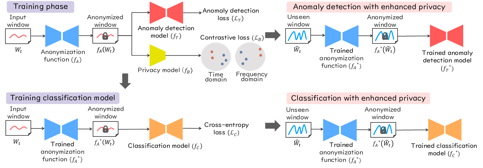
The proposed framework comprises an anonymization function \(f_A\) for time-series data, a privacy model \(f_B\), and an anomaly-detection model \(f_{T}\), which collectively contribute to the training of \(f_A\), as illustrated in Fig. 1. \(f_A\) transforms the time series by removing information that compromises privacy while retaining information essential for accurate anomaly detection. We train \(f_A\) using a combined loss function that incorporates a contrastive loss, \(\mathcal{L}_{B}\), derived from \(f_B\), and an anomaly detection loss, \(\mathcal{L}_{T}\), derived from \(f_T\). During training, \(f_A\) learns to preserve information relevant to anomaly detection, guided by \(\mathcal{L}_{T}\). Simultaneously, \(f_A\) and \(f_B\) are trained adversarially using \(\mathcal{L}_{B}\) to ensure that \(f_A\) effectively removes sensitive information from the time-series data. By employing the anonymization function \(f_A\), trained in this manner, we can achieve anomaly detection that maintains both privacy and high performance.
After training \(f_A\), \(f_B\), and \(f_T\), we train a classification model, \(f_C\), using a cross-entropy loss, \(\mathcal{L}_{C}\), to evaluate the effectiveness of the anonymization achieved by the trained \(f_A\) (Section 3.6).
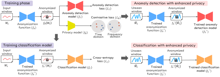
Fig. 1. Anomaly-detection framework with enhanced privacy. The anonymization function, \(f_{A}\), transforms a time series window, \(W_{t}\). Through adversarial training with a privacy model (\(f_{B}\)) using contrastive loss and an anomaly-detection model (\(f_{T}\)) using anomaly detection loss, \(f_{A}\) learns to remove sensitive information from \(W_{t}\) while preserving features essential for anomaly detection.
3.1. Problem Formulation
A time series is a sequence of data points representing the observed state of a particular subject over time. Time series can be categorized into univariate, comprising a single feature, and multivariate, comprising multiple features. Each feature in a multivariate time series can be considered an individual univariate time series. Let a time series consist of \(M\) data points: \(\mathcal{X} = \{\mathbf{x}_{1}, \mathbf{x}_{2}, \ldots, \mathbf{x}_{M}\}\), where each data point \(\mathbf{x}_{t} \in \mathbb{R}^{D}\) is collected at a specific timestep \(t\). Here, \(D\) (\(D\geq1\)) represents the number of features. In this study, \(\mathcal{X}\) is converted into a series of windows \(\mathcal{X}=\{W_{1}, W_{2}, W_{3}, \ldots\}\), and the framework operates on these window units. Each window comprises \(L\) data points, represented as \(W_{t}=\{\mathbf{x}_{t}, \mathbf{x}_{t+1}, \ldots, \mathbf{x}_{t+L-1}\}\).
In the context of anomaly detection with enhanced privacy, when \(f_{A}\) receives a set of unseen windows for testing, denoted as \(\mathcal{X}_{test}=\{\hat{W}_{1}, \hat{W}_{2}, \hat{W}_{3},\ldots\}\), it generates an anonymized version, \(f_{A}^{*}(\hat{W}_{t})\), for each \(\hat{W}_{t}\) using the trained \(f_{A}^{*}\). This anonymized output, \(f_{A}^{*}(\hat{W}_{t})\), is then fed into the trained \(f^{*}_T\), which determines whether the original \(\hat{W}_{t}\) contains an anomaly. To evaluate the anomaly-detection performance, a corresponding set of labels, \(\mathcal{Y}_{test}=\{y_{1}, y_{2}, y_{3},\ldots\}\), is used to access whether each \(y_{t}\) is correctly predicted for \(\hat{W}_{t}\). Here, \(y_{t} \in \{0, 1\}\), and \(\hat{W}_{t}\) is considered anomalous if \(y_{t}=1\) and normal if \(y_{t}=0\).
The overarching goal of anomaly detection with enhanced privacy is to maintain sufficient accuracy in practical applications, even when operating on time series with robust privacy preservation. This goal is achieved by constructing an anonymization function, \(f_{A}\), that satisfies the following two criteria:
-
・
\(f_{A}\) does not significantly impact the performance of anomaly detection. That is, anomaly detection using time-series data anonymized by \(f_{A}\) should achieve accuracy comparable to that of anomaly detection using the original, non-anonymized data.
-
・
\(f_{A}\) effectively removes sensitive information, such as contextual features and PII, from the time series.
3.2. Anomaly Detection Model \(\boldsymbol{f_T}\)
In this study, we employ the an anomaly transformer 32 as our anomaly detection model, \(f_{T}\). The Anomaly Transformer uses a specialized “Anomaly-Attention” mechanism to quantify the relationships between data points in a time series. Based on these relationships, it evaluates the degree to which each data point deviates from normal patterns (discrepancy) to detect anomalies. The model is trained on only normal time-series data to learn the underlying patterns of normality. During the anomaly-detection phase, it can identify anomalies based on deviations from this learned normality.
The anomaly-detection model, \(f_{T}\), is trained to minimize the loss function \(\mathcal{L}_{T}\). Furthermore, \(\mathcal{L}_{T}\) is also used in the training of the anonymization function, \(f_{A}\), with \(f_{A}\) being trained to minimize this value similarly to \(f_{T}\). Consequently, \(f_{A}\) enables anonymization that preserves valuable information for anomaly detection, and \(f_{T}\) enables highly accurate anomaly detection using the anonymized data.
3.3. Privacy Model \(\boldsymbol{f_B}\)
In this study, the objective of the privacy model \(f_B\) is to explicitly identify the information that should be removed by the anonymization function \(f_A\). Specifically, \(f_B\) is designed to extract sensitive information, including PII and contextual features embedded in the time series. Importantly, \(f_B\) is not used during the final inference. Instead, it serves as an auxiliary model that guides the training of \(f_A\). By adversarially suppressing the information that \(f_B\) seeks to retain, \(f_A\) enhances privacy.
We trained the anonymization function \(f_A\) and privacy model \(f_B\) adversarially within a min-max optimization framework. In general, adversarial training optimizes a shared loss function in opposite directions across models 40,41. One model minimizes the loss, while the other maximizes it, establishing a competitive relationship. Through iterative optimization, \(f_B\) learns to extract sensitive semantic information, whereas \(f_A\) learns to suppress it. Consequently, removable information is attenuated, and only task-relevant information is retained. Fig. 2 illustrates the adversarial framework between \(f_A\) and \(f_B\).
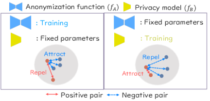
Fig. 2. \(f_A\) and \(f_B\) are adversarially trained using a shared contrastive loss.
A key element in adversarial training is the shared loss function. In this study, we adopted contrastive loss as the common objective. Contrastive learning 42 is a self-supervised method that learns structured representations in an embedding space without explicit labels. It pulls positive pairs closer together while pushing negative pairs apart. Positive pairs are generated from different augmentations of the same time-series instance, whereas negative pairs are constructed from distinct time-series or temporally distant samples. For positive-pair generation, we employed augmentation techniques commonly used in contrastive learning, including jittering, scaling, time shifts, and neighborhood segmentation 42,43. Negative pairs are formed from different time series within the same batch. Through this process, the model emphasizes semantic information that distinguishes positive from negative pairs, learning discriminative representations. We define the contrastive loss \(\mathcal{L}_B\) using the normalized temperature-scaled cross-entropy loss (NT-Xent) 42.
During training, we alternately update \(f_B\) and \(f_A\). When updating \(f_B\), the parameters of \(f_A\) are fixed, and we minimize \(\mathcal{L}_B\). This encourages \(f_B\) to retain information that is useful for distinguishing between positive and negative pairs. Conversely, when updating \(f_A\), the parameters of \(f_B\) are fixed, and \(\mathcal{L}_B\) is maximized. This compels \(f_A\) to suppress the information \(f_B\) relies on to discriminate between samples. In other words, by treating contrastive loss, our method selectively removes information that facilitates discrimination between positive and negative pairs. In time-series data, such discriminative information may correspond to semantic features, such as shape-related patterns or PII.
The objective of \(f_A\) is not merely to remove information. In addition to adversarial optimization, \(f_A\) is trained to minimize the anomaly detection loss \(\mathcal{L}_T\) described in Section 3.2. This joint objective ensures that only information emphasized by contrastive learning, and irrelevant to anomaly detection, is attenuated, while information essential for accurate detection is preserved through \(\mathcal{L}_T\).
In time-series contrastive learning, representations are typically learned in the time domain 44,45,46,47,48,49,50. Following 51, we extend contrastive learning to both time and frequency domains. Incorporating frequency-domain representations enables the model to capture periodic and structural patterns that may not be evident in the time domain. This dual-domain contrastive framework allows \(f_B\) to extract a broader set of discriminative features, which are then adversarially suppressed by \(f_A\). Leveraging both domains is therefore critical for stronger privacy preservation. The final \(\mathcal{L}_B\) value is the sum of Eqs. (10) and (11) in Appendix G.
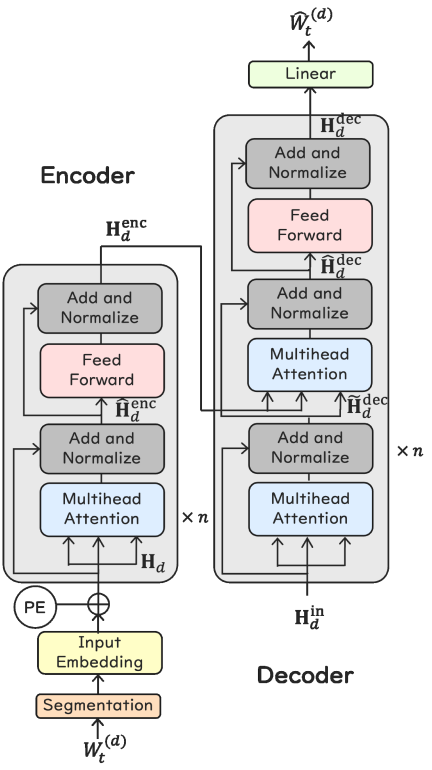
Fig. 3. Feature-independent encoder–decoder architecture of \(f_A\), illustrated for a single feature \(d\) (\(1 \leq d \leq D\)).
3.4. Anonymization Function \(\boldsymbol{f_A}\)
This section introduces the architecture and training procedure of the anonymization function, \(f_A\).
Segmentation. Segmentation is a technique that groups data points with similar characteristics, treating them as a single unit. This is particularly effective for time-series data because temporally adjacent data points often exhibit similar characteristics 38,52. By performing segmentation, we can determine local temporal patterns and dependencies between data points, allowing for a more precise capture of the characteristics of the time series. In this study, we adopted segmentation in the design of \(f_{A}\), processing input windows by dividing them into segments.
Operation in the Transformer Module. Time-series data inherently exhibit temporal dependencies between data points, and capturing this contextual information is crucial for improving the accuracy of downstream tasks 52. Therefore, we used the transformer architecture for \(f_{A}\), as it excels in capturing contextual information. Generally, when a transformer handles multivariate time series, it aggregates information across all features into a unified representation. However, because each feature in a multivariate time series often carries different meanings and importance, it is desirable to perform anonymization on a dimension-by-dimension basis. Therefore, in this study, we performed anonymization using feature-independent encoder–decoder networks. The overall architecture is illustrated in Fig. 3. The parameters were updated with feature-specific gradient magnitudes derived from \(\mathcal{L}_B\) and \(\mathcal{L}_T\), enabling differential suppression or preservation of information across features. This approach allows for more precise anonymization and preservation of important information specific to each feature in the time series.
Encoder Design. When the encoder receives an input window \(W_{t} \in \mathbb{R}^{L \times D}\), each feature \(W_t^{(d)} \in \mathbb{R}^{L}\) (\(1 \leq d \leq D\)) is independently segmented and linearly projected, then added with a positional embedding, producing the per-feature representation \(\mathbf{H}_{d} \in \mathbb{R}^{N \times d_\text{model}}\). Here, \(N\) denotes the number of segments and \(d_\text{model}\) denotes the embedding dimensionality. The encoder then performs multihead attention in the time direction to capture the temporal dependencies of the input time series. After the multihead attention (\(\operatorname{ATTN}\)), we obtain the output:
Decoder Design. The decoder performs anonymization by referring to the output \(\mathbf{H}_{d}^{\text{enc}, l}\) of layer \(l\) of the encoder as follows:
The final per-feature output \(\widehat{W}_t^{(d)} \in \mathbb{R}^{L}\) is expressed as
Training of \(\boldsymbol{f_A}\). \(f_{A}\) is trained to minimize \(\mathcal{L}_{T}\) and maximize \(\mathcal{L}_{B}\). This approach allows \(f_{A}\) to effectively anonymize data by removing sensitive information while preserving the information necessary for anomaly detection.
3.5. Overall Training Flow
The proposed framework involves three models: the anonymization function \(f_{A}\), anomaly detection model \(f_{T}\), and privacy model \(f_{B}\), parameterized by \(\theta_{A}\), \(\theta_{T}\), and \(\theta_{B}\), respectively. Let \(\alpha_{A}\), \(\alpha_{T}\), and \(\alpha_{B}\) be the learning rates for \(\theta_{A}\), \(\theta_{T}\), and \(\theta_{B}\), respectively. The training procedure comprises an alternating optimization scheme with two main steps:
-
1.
Learning of \(\boldsymbol{f_A}\): This step focuses solely on updating the parameters \(\theta_{A}\) of \(f_{A}\). The objective is to minimize the anomaly detection loss, \(\mathcal{L}_{T}\), and simultaneously maximize the contrastive loss, \(\mathcal{L}_{B}\).
\begin{equation} \label{eq:eqnU003Afa} \theta_A \leftarrow \theta_A-\alpha_A \nabla_{\theta_A}\left(\mathcal{L}_T\left(\theta_A, \theta_{T}\right)-\mathcal{L}_B\left(\theta_A, \theta_B\right)\right). \tag{5} \end{equation} -
2.
Learning \(\boldsymbol{f_T}\) and \(\boldsymbol{f_B}\): In this step, \(\theta_{T}\) and \(\theta_{B}\) of \(f_{T}\) and \(f_{B}\) are updated, where \(\mathcal{L}_{T}\) and \(\mathcal{L}_{B}\) are used to train \(f_{T}\) and \(f_{B}\), respectively.
\begin{equation} \label{eq:eqnU003Afbandft} \left\{ \begin{aligned} & \theta_T \leftarrow \theta_{T}-\alpha_{T} \nabla_{\theta_{T}}\left(\mathcal{L}_{T}\left(\theta_{T}, \theta_A\right)\right), \\ & \theta_B \leftarrow \theta_B-\alpha_B \nabla_{\theta_B}\left(\mathcal{L}_B\left(\theta_B, \theta_A\right)\right) . \end{aligned} \right. \tag{6} \end{equation}
By minimizing \(\mathcal{L}_{T}\) as shown in Eq. (5), \(f_{A}\) learns to anonymize the data within the input window while preserving information crucial for accurate anomaly detection. Concurrently, \(f_{T}\) is trained to minimize \(\mathcal{L}_{T}\) using Eq. (6), enhancing its ability to detect anomalies in the anonymized data. The adversarial training between \(f_{A}\) and \(f_{B}\) is facilitated through \(\mathcal{L}_{B}\): maximizing \(\mathcal{L}_{B}\) with respect to \(f_{A}\) in Eq. (5) and minimizing it with respect to \(f_{B}\) in Eq. (6) creates a competitive dynamic. This competition enables \(f_{A}\) to learn an anonymization function that effectively removes sensitive information that \(f_{B}\) focuses on, thereby enhancing privacy.
3.6. Classification Model \(\boldsymbol{f_C}\)
Previous studies on anonymization have primarily focused on evaluating the trade-off between the strength of anonymization (e.g., the amount of noise added) and the performance of downstream tasks such as anomaly detection. However, the sufficiency of anonymization in terms of removing specific sensitive information, such as PII, from time-series data has not been thoroughly investigated. To address this gap, we quantitatively evaluated the sufficiency of anonymization using a time-series dataset where each window was assigned a unique ID. These IDs were represented as trainable embedding vectors and appended to the original windows. Anonymization was then performed on data within these windows with the appended ID vectors.
To assess the effectiveness of anonymization in removing ID-related information, we trained a separate classification model, \(f_{C}\), based on the transformer architecture. This model attempts to predict the correct ID from the anonymized window generated by \(f_{A}^{*}\). A low classification accuracy indicates that \(f_{A}^{*}\) has successfully removed the identifying information. Conversely, a high classification accuracy suggests insufficient anonymization, as ID-related information is still present in the anonymized data. \(f_{C}\) is trained using the cross-entropy loss, \(\mathcal{L}_{C}\), as in 53. \(\mathcal{L}_{C}\) is defined as
4. Experiments
This section details the experiments conducted to evaluate the proposed framework for anomaly detection with enhanced privacy using datasets containing PII. We assessed anonymization sufficiency and anomaly-detection accuracy.
4.1. Datasets and Preprocessing
We conducted our experiments using four datasets widely used in anomaly detection studies: ECG 54,55, TODS 56, SWaT 57, and PSM 58.
ECG contains an electrocardiogram (ECG) time series from 47 subjects, including both normal and irregular heartbeats (arrhythmias). We removed duplicate data and data of those using pacemakers, resulting in a dataset of 41 unique subjects. For anomaly detection, we evaluated arrhythmia-detection accuracy from the anonymized ECG data. We then assessed whether the anonymized heartbeats could be used to classify the 41 subjects as a measure of anonymization sufficiency.
TODS is a synthetic time series dataset generated using the method proposed in 56. We created five types of five-dimensional time series, each with distinct function types (e.g., sine and cosine functions), frequencies, and amplitudes. We assigned a unique ID to each of the five types. Following the anomaly classification in 56, which categorizes anomalies into point-wise (global and contextual) and pattern-wise (seasonal, group, and trend) anomalies, we inserted both point-wise and pattern-wise anomalies into the TODS test data.
SWaT and PSM are widely used datasets for anomaly detection in multivariate time series. Unlike the ECG dataset, the original SWaT and PSM datasets do not contain sensitive information. Therefore, to evaluate anonymization effectiveness, we randomly assigned 50 unique IDs to windows in both the training and test sets of each dataset.
As a preprocessing step, we applied standardization, a common technique in time series analysis, to transform the data to a common scale 59. We standardized both the training and test data using the mean and standard deviation of the training data only. Each data point \(\mathbf{x}_{t}\) was transformed as follows:
4.2. Evaluation Metrics
Anomaly-detection performance. Following 60, we used the point-wise F1 score, precision, and recall to evaluate anomaly-detection performance. In this context, a predicted anomaly is considered valid if it falls within a specific margin of the actual location of the anomaly. This acknowledges that slight deviations in the precise timing of anomaly detection may still be acceptable. A critical aspect of anomaly detection is the selection of a threshold for the anomaly score, above which a data point or window is classified as anomalous. However, the anomaly-detection performance can be highly sensitive to the selected threshold 60. To eliminate the influence of threshold selection and ensure a fair comparison, we report the best F1 score, which is obtained using the threshold that yields the highest F1 score across all methods for each dataset.
Time-Series Similarity under Anonymization. To evaluate the effectiveness of anonymization in removing contextual features from the original time series, we measured the similarity between the original time series window, \(W_{t}\), and its anonymized counterpart, \(\hat{W}_{t}\), using normalized cross-correlation (NCC) 61. Previous work demonstrated that NCC is a robust and computationally efficient similarity metric for time series 62. NCC computes the cross-correlation sequence, \(CC(W_{t}, \hat{W}_{t})\), between two windows \(W_{t}\) and \(\hat{W}_{t}\), and then normalizes it by the product of their Euclidean norms:
PII Removal through Anonymization. We evaluated the effectiveness of PII removal, specifically the removal of ID information embedded in the time series, using the classification model, \(f_{C}\), as described in Section 3.6. The anonymized window is fed as input to \(f_{C}\), which then performs a classification task to predict the ID associated with that window. Low accuracy in this classification task indicates that the ID information has been effectively removed from the window through anonymization, thus achieving the desired privacy goal.
4.3. Anonymization Methods
We compared the proposed framework against five baseline anonymization methods based on DP, as introduced in Section 2.
Laplace mechanism directly modifies the original data values by adding noise drawn from a Laplace distribution.
Temporal perturbation perturbs the temporal information by dispersing data points within the same window to different timestamps.
DP-SGD is an optimization framework that adapts the stochastic gradient descent method 63,64 to satisfy DP. In this context, we trained the anonymization function, \(f_{A}\), using the DP-SGD algorithm. This algorithm clips the gradients of the parameters to a fixed norm (gradient clipping) and adds Gaussian noise to the clipped gradients. Gradient clipping limits the influence of excessively large gradients on parameter updates, thus bounding the sensitivity of the updates to individual data points. The anonymized data were then generated using the trained \(f_{A}\).
DP-Adam learns \(f_{A}\) using Adam 65 instead of SGD in DP-SGD.
DP-AdaGrad learns \(f_{A}\) using AdaGrad 66 instead of SGD in DP-SGD.
4.4. Experimental Setup
For a fair comparison, the experimental settings were consistent across all anonymization methods. We set the window length to 50, batch size to 128, and number of epochs to 10. We employed the Adam optimizer for training. All experiments were performed three times, and the means of the evaluation metrics are reported. For the baseline anonymization methods, we replaced the \(f_{A}\) component in the proposed framework with each respective method while retaining the anomaly transformer for \(f_{T}\). Notably, the privacy model, \(f_{B}\), was not used in these baseline methods. Laplace mechanism samples noise from a Laplace distribution with a mean of 0 and variance of 1, as described in 19. Temporal perturbation employs a sliding window length of 10 for dispersing data points, as specified in 21. In DP-SGD, DP-Adam, and DP-AdaGrad, noise is sampled from a Gaussian distribution with a mean of 0 and variance of 2, and the clipping threshold was set to 4, as detailed in 24. For DP-SGD, DP-Adam, and DP-AdaGrad, we used Transformers for \(f_{A}\). We used SGD as the optimizer to train \(f_{A}\) in DP-SGD and AdaGrad as the optimizer to train \(f_{A}\) in DP-AdaGrad.
| Method | ECG | TODS | SWaT | PSM | ||||||||||||||||
| Anomaly detection | Privacy | Anomaly detection | Privacy | Anomaly detection | Privacy | Anomaly detection | Privacy | |||||||||||||
| Metric | Pre | Rec | F1 (↑) | NCC (↓) | Acc (↓) | Pre | Rec | F1 (↑) | NCC (↓) | Acc (↓) | Pre | Rec | F1 (↑) | NCC (↓) | Acc (↓) | Pre | Rec | F1 (↑) | NCC (↓) | Acc (↓) |
| Raw data | 46.4 | 84.0 | 57.8 | – | 65.5 | 77.2 | 100.00 | 87.1 | – | 84.9 | 99.3 | 61.2 | 76.0 | – | 65.3 | 44.2 | 73.1 | 55.1 | – | 77.4 |
| Laplace mechanism | 35.3 | 100.0 | 52.1 | 0.60 | 53.1 | 69.6 | 100.00 | 82.1 | 0.65 | 82.3 | 99.4 | 60.6 | 75.3 | 0.52 | 63.2 | 32.0 | 100.0 | 48.0 | 0.55 | 68.3 |
| Temporal perturbation | 35.3 | 100.0 | 52.1 | 0.69 | 64.5 | 73.5 | 100.00 | 84.7 | 0.36 | 47.6 | 47.9 | 60.3 | 39.9 | 0.77 | 55.2 | 32.3 | 100.0 | 48.8 | 0.75 | 68.2 |
| DP-SGD | 36.5 | 94.1 | 52.4 | 0.90 | 61.4 | 75.8 | 100.00 | 86.3 | 0.50 | 45.7 | 52.0 | 68.8 | 53.3 | 0.49 | 48.9 | 29.4 | 97.4 | 45.1 | 0.43 | 43.9 |
| DP-Adam | 36.7 | 93.0 | 52.6 | 0.91 | 63.8 | 75.9 | 100.00 | 86.3 | 0.51 | 50.9 | 63.4 | 60.6 | 61.4 | 0.50 | 44.2 | 29.9 | 96.2 | 45.5 | 0.43 | 38.6 |
| DP-AdaGrad | 35.9 | 96.8 | 52.4 | 0.89 | 60.9 | 75.7 | 100.00 | 86.1 | 0.50 | 46.1 | 68.4 | 62.4 | 64.7 | 0.49 | 42.4 | 29.2 | 100.0 | 45.2 | 0.43 | 43.8 |
| Ours | 40.5 | 87.1 | 53.3 | 0.21 | 31.2 | 76.2 | 100.00 | 86.4 | 0.33 | 18.7 | 99.4 | 61.6 | 76.0 | 0.25 | 35.2 | 34.7 | 89.7 | 50.0 | 0.20 | 37.4 |
4.5. Results
Table 1 summarizes the results of our evaluation, focusing on both the sufficiency of anonymization and anomaly-detection performance. Each experiment was conducted three times under each setting, and the reported values represent the mean performance across runs. The standard deviations of each metric over three runs are reported in Table 7 (in Appendix A.4). Across all datasets, the proposed framework achieved the lowest NCC and ID-classification accuracy of all compared anonymization methods while incurring only a minor average reduction of 2.58% in the F1 score for anomaly detection. The proposed framework demonstrated a low similarity between pre- and post-anonymized time series, with NCC values ranging from 0.20 to 0.33. This indicates that the anonymization function, \(f_{A}\), effectively removes the contextual features of the original time series. This success can be attributed to the adversarial training process using contrastive loss, which allows \(f_{A}\) to eliminate the features of the original time series that are targeted by the privacy model, \(f_{B}\).
Furthermore, we achieved a 42.65% reduction in ID-classification accuracy, averaged across all datasets. Compared to existing anonymization methods, the proposed framework demonstrates significantly lower accuracy in classifying the ID of each window. Notably, the ID-classification accuracy dropped by more than 30 percentage points. This is because \(f_{A}\) not only removes features related to time series but also effectively eliminates ID-related information from the windows. The adversarial training process, incorporating contrastive loss, is crucial in erasing ID-related information targeted by \(f_{B}\).
Importantly, the F1-scores for anomaly-detection indicate that even with sufficiently anonymized time series, anomaly-detection accuracy is not significantly degraded compared to using the original raw data. This is because \(f_{A}\) is trained using a combination of anomaly detection and contrastive losses, ensuring that information useful for anomaly detection is retained within the anonymized window. Therefore, the proposed framework successfully detects anomalies while maintaining performance by preserving the necessary information.
5. Analysis
5.1. Contrastive Loss in Time-Frequency Domain
As described in Section 3.3, we removed sensitive information from the time series through the adversarial training of \(f_{A}\) and \(f_{B}\) using contrastive loss. Furthermore, we applied contrastive loss in the time and frequency domains. Incorporating representations from the frequency domain allows capturing semantic information regarding the time series that may be overlooked when considering only the time domain. This approach ensures robust anonymization by effectively removing sensitive information through representations in both time and frequency domains. To evaluate the effectiveness of this dual-domain approach, we compared the performance of our framework using three different configurations: time domain, frequency domain, and a combination of time and frequency domains TF-domain, on the ECG, TODS, SWaT, and PSM datasets. We analyzed the impact on NCC, ID-classification accuracy, and F1-score for anomaly detection.
Table 2 shows the results of this comparison. We observe that for all datasets, using TF-domain results in an average decrease of 0.025 in NCC and a 2–11 percentage point drop in ID-classification accuracy compared to using time domain and frequency domain alone. Additionally, the highest average F1-score for anomaly detection is achieved by combining the time and frequency domains.
| Domain | ECG | TODS | SWaT | PSM | ||||||||
| Anomaly | Privacy | Anomaly | Privacy | Anomaly | Privacy | Anomaly | Privacy | |||||
| Metric | F1 (↑) | NCC (↓) | Acc (↓) | F1 (↑) | NCC (↓) | Acc (↓) | F1 (↑) | NCC (↓) | Acc (↓) | F1 (↑) | NCC (↓) | Acc (↓) |
| Time domain | 53.2 | 0.18 | 35.7 | 83.8 | 0.34 | 27.8 | 75.9 | 0.29 | 46.4 | 47.6 | 0.38 | 40.0 |
| Frequency domain | 53.1 | 0.19 | 34.9 | 82.7 | 0.35 | 26.4 | 75.9 | 0.41 | 48.9 | 48.1 | 0.42 | 46.2 |
| TF-domain | 53.3 | 0.21 | 31.2 | 86.4 | 0.33 | 18.7 | 76.0 | 0.25 | 35.2 | 50.0 | 0.36 | 37.4 |
5.2. Effect of Components
To investigate the contribution of each component in the proposed framework, we conducted ablation studies by removing the privacy model \(f_B\) (w/o \(f_B\)) and the adversarial training mechanism (w/o adversarial training). These variants allow us to isolate the individual effects of \(f_B\) and adversarial optimization on overall performance. The results are presented in Table 3.
As shown in Table 3, the proposed framework, incorporating both \(f_B\) and adversarial training, achieved superior performance in terms of both anomaly detection and privacy preservation. Notably, NCC and ID-classification accuracies showed substantial improvement. These findings indicate that \(f_B\) plays a crucial role in guiding the anonymization of \(f_A\), and that adversarial training enhances the ability of \(f_A\) to identify and suppress sensitive information through competitive optimization.
| Domain | ECG | TODS | SWaT | PSM | ||||||||
| Anomaly | Privacy | Anomaly | Privacy | Anomaly | Privacy | Anomaly | Privacy | |||||
| Metric | F1 (↑) | NCC (↓) | Acc (↓) | F1 (↑) | NCC (↓) | Acc (↓) | F1 (↑) | NCC (↓) | Acc (↓) | F1 (↑) | NCC (↓) | Acc (↓) |
| w/o \(\boldsymbol{f_B}\) | 52.1 | 0.29 | 48.0 | 78.4 | 0.58 | 73.6 | 75.7 | 0.28 | 54.4 | 48.0 | 0.45 | 51.6 |
| w/o adversarial training | 52.1 | 0.28 | 48.4 | 79.0 | 0.56 | 52.2 | 75.9 | 0.32 | 41.4 | 47.2 | 0.38 | 46.7 |
| Ours | 53.3 | 0.21 | 31.2 | 86.4 | 0.33 | 18.7 | 76.0 | 0.25 | 35.2 | 50.0 | 0.36 | 37.4 |
5.3. Qualitative Analysis
Figure 4 illustrates examples of ECG from multiple subjects anonymized using the proposed framework and existing anonymization methods.
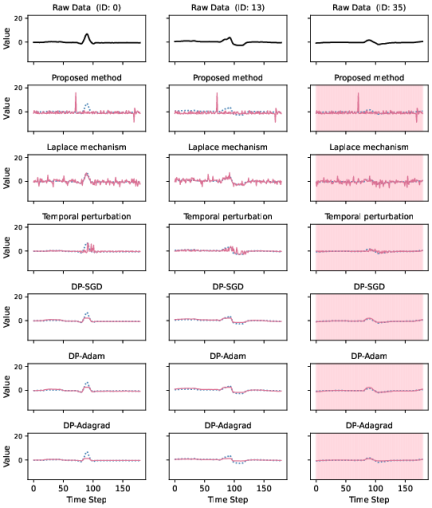
Fig. 4. Examples of anonymized time series. Whereas existing anonymization methods retain the original contextual features of the time series, the proposed framework successfully removes them.
The first row (black solid line) represents the original raw data. The subsequent rows show the time series before (blue dotted line) and after (pink solid line) anonymization using different methods. The red-highlighted ECG (subject ID 35) indicates an arrhythmia (abnormality). Existing methods, which primarily rely on adding noise, introduce slight differences in individual data points compared to the original values. However, they generally preserve the characteristic shape of the original time series after anonymization. In contrast, the proposed framework significantly alters the characteristic shape, making windows from different subjects appear more similar and difficult to distinguish. Although anonymized ECGs with arrhythmias may be more challenging for humans to interpret visually, the proposed framework retains information critical for anomaly detection, thus maintaining detection performance. These results demonstrate that the proposed framework enables effective anomaly detection with enhanced privacy by removing identifiable patterns while preserving essential features for anomaly detection.
5.4. Visualization of Anonymized Sensitive Data
As mentioned in Section 3.3, the trained \(f_{A}\) removes ID-related information. To visually confirm this, we created scatter plots of window vectors in the ECG test data using t-SNE 67. Fig. 5(a) shows the scatter plot of the raw data, and Fig. 5(b) shows that of the data anonymized by \(f_{A}\). Plots with the same color indicate the same ID. The visualization results for other anonymization methods are presented in Appendix E. In the raw data, each window retains its ID, resulting in window vectors being grouped by ID, forming distinct clusters. In contrast, the anonymized data demonstrates that the window vectors are not organized into clusters but are instead intermixed. This indicates that \(f_{A}\) effectively removed ID-related information from the windows and such information is absent from the window vectors. These results demonstrate that the proposed framework effectively removes sensitive information unrelated to anomaly detection from time series using \(f_{A}\).
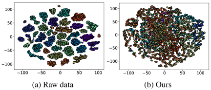
Fig. 5. Scattergram of window vectors by ID, visualized using t-SNE. Plots with the same color indicate the same ID. The proposed framework successfully removes ID-related information from the time series.
6. Conclusions
In this study, we developed a novel framework for privacy-preserving anomaly detection in time-series data. Our framework successfully addresses the inherent trade-off between the sufficiency of privacy preservation and accuracy of anomaly detection. To achieve this balance, we introduced an anonymization function trained through an adversarial process. This function uses contrastive loss to remove sensitive information, including contextual features and PII, while simultaneously employing anomaly detection loss to preserve the information essential for accurate anomaly detection. Experimental results demonstrate that our framework effectively anonymizes time-series data, eliminating the original contextual features and PII, while maintaining anomaly-detection performance comparable to that achieved using the original, non-anonymized data.
This study focused on anomaly detection. Therefore, future work should aim to construct a more versatile framework applicable to a wider range of time-series analysis tasks, further expanding the potential for privacy-preserving data analysis.
Acknowledgments
This work was supported by JSPS KAKENHI Grant Number JP24999361 (Grant-in-Aid for Early-Career Scientists).
- [1] A. A. Cook, G. Mısırlı, and Z. Fan, “Anomaly detection for IoT time-series data: A survey,” IEEE Internet of Things J., Vol.7, No.7, pp. 6481-6494, 2020. https://doi.org/10.1109/JIOT.2019.2958185
- [2] G. Pang, C. Shen, L. Cao, and A. V. D. Hengel, “Deep learning for anomaly detection: A review,” ACM Computing Surveys (CSUR), Vol.54, No.2, pp. 1-38, 2021. https://doi.org/10.1145/3439950
- [3] M. Landauer, S. Onder, F. Skopik, and M. Wurzenberger, “Deep learning for anomaly detection in log data: A survey,” Machine Learning with Applications, Vol.12, Article No.100470, 2023. https://doi.org/10.1016/j.mlwa.2023.100470
- [4] Y. Mao, Q. Ye, Q. Wang, and H. Hu, “Differential Privacy for Time Series: A Survey,” IEEE Data Eng. Bull., Vol.48, No.2, pp. 67-92, 2024.
- [5] X. Zhang, C. Chen, Y. Xie, X. Chen, J. Zhang, and Y. Xiang, “A survey on privacy inference attacks and defenses in cloud-based deep neural network,” Computer Standards & Interfaces, Vol.83, Article No.103672, 2023. https://doi.org/10.1016/j.csi.2022.103672
- [6] M. Al-Rubaie and J. M. Chang, “Privacy-preserving machine learning: Threats and solutions,” IEEE Security & Privacy, Vol.17, No.2, pp. 49-58, 2019. https://doi.org/10.1109/MSEC.2018.2888775
- [7] S. Sagiroglu and D. Sinanc, “Big data: A review,” 2013 Int. Conf. on Collaboration Technologies and Systems (CTS), pp. 42-47, 2013. https://doi.org/10.1109/CTS.2013.6567202
- [8] M. Keshk, E. Sitnikova, N. Moustafa, J. Hu, and I. Khalil, “An integrated framework for privacy-preserving based anomaly detection for cyber-physical systems,” IEEE Trans. on Sustainable Computing, Vol.6, No.1, pp. 66-79, 2021. https://doi.org/10.1109/TSUSC.2019.2906657
- [9] I. Makhdoom, M. Abolhasan, J. Lipman, N. Shariati, D. Franklin, and M. Piccardi, “Securing Personally Identifiable Information: A Survey of SOTA Techniques, and a Way Forward,” IEEE Access, Vol.12, pp. 116740-116770, 2024. https://doi.org/10.1109/ACCESS.2024.3447017
- [10] A. Machanavajjhala, J. Gehrke, D. Kifer, and M. Venkitasubramaniam, “L-diversity: Privacy beyond k-anonymity,” 22nd Int. Conf. on Data Engineering (ICDE’06), pp. 24-24, 2006. https://doi.org/10.1109/ICDE.2006.1
- [11] S. Mehnaz and E. Bertino, “Privacy-preserving Real-time Anomaly Detection Using Edge Computing,” 2020 IEEE 36th Int. Conf. on Data Engineering (ICDE), pp. 469-480, 2020. https://doi.org/10.1109/ICDE48307.2020.00047
- [12] N. Gruver, M. Finzi, S. Qiu, and A. G. Wilson, “Large Language Models Are Zero-Shot Time Series Forecasters,” Advances in Neural Information Processing Systems, Vol.36, pp. 19622-19635, 2023.
- [13] M. Goswami, K. Szafer, A. Choudhry, Y. Cai, S. Li, and A. Dubrawski, “MOMENT: A Family of Open Time-series Foundation Models,” Int. Conf. on Machine Learning, pp. 16115-16152, 2024.
- [14] X. Shi, S. Wang, Y. Nie, D. Li, Z. Ye, Q. Wen, and M. Jin, “Time-MoE: Billion-Scale Time Series Foundation Models with Mixture of Experts,” arXiv preprint, arXiv:2409.16040, 2024. https://doi.org/10.48550/arXiv.2409.16040
- [15] K. K. Nakka, A. Frikha, R. Mendes, X. Jiang, and X. Zhou, “PII-Scope: A Comprehensive Study on Training Data PII Extraction Attacks in LLMs,” arXiv preprint, arXiv:2410.06704, 2024. https://doi.org/10.48550/arXiv.2410.06704
- [16] H. Li, D. Guo, W. Fan, M. Xu, J. Huang, F. Meng, and Y. Song, “Multi-step Jailbreaking Privacy Attacks on ChatGPT,” Findings of the Association for Computational Linguistics: EMNLP 2023, 2023. https://doi.org/10.18653/v1/2023.findings-emnlp.272
- [17] C. Dwork, “Differential privacy,” Int. Colloquium on Automata, Languages, and Programming, 2006. https://doi.org/10.1007/11787006_1
- [18] V. Rastogi and S. Nath, “Differentially private aggregation of distributed time-series with transformation and encryption,” Proc. of the 2010 ACM SIGMOD Int. Conf. on Management of Data, pp. 735-746, 2010. https://doi.org/10.1145/1807167.1807247
- [19] J. W. Kim, B. Jang, and H. Yoo, “Privacy-preserving aggregation of personal health data streams,” PloS One, Vol.13, No.11, Article No.e0207639, 2018. https://doi.org/10.1371/journal.pone.0207639
- [20] Q. Ye, H. Hu, N. Li, X. Meng, H. Zheng, and H. Yan, “Beyond Value Perturbation: Local Differential Privacy in the Temporal Setting,” IEEE Conf. on Computer Communications (IEEE INFOCOM 2021), 2021. https://doi.org/10.1109/INFOCOM42981.2021.9488899
- [21] Q. Ye, H. Hu, K. Huang, M. H. Au, and Q. Xue, “Stateful Switch: Optimized Time Series Release with Local Differential Privacy,” IEEE Conf. on Computer Communications (IEEE INFOCOM 2023), 2023. https://doi.org/10.1109/INFOCOM53939.2023.10229063
- [22] Y. Mao, Q. Ye, Q. Wang, and H. Hu, “Utility-Aware Time Series Data Release With Anomalies Under TLDP,” IEEE Trans. on Mobile Computing, Vol.23, No.6, pp. 7135-7147, 2024. https://doi.org/10.1109/TMC.2023.3332963
- [23] G. Giorgi, W. Abbasi, and A. Saracino, “Privacy-Preserving Analysis for Remote Video Anomaly Detection in Real Life Environments,” J. Wirel. Mob. Networks Ubiquitous Comput. Dependable Appl., Vol.13, No.1, pp. 112-136, 2022. https://doi.org/10.22667/JOWUA.2022.03.31.112
- [24] M. Abadi, A. Chu, I. Goodfellow, H. B. McMahan, I. Mironov, K. Talwar, and L. Zhang, “Deep learning with differential privacy,” Proc. of the 2016 ACM SIGSAC Conf. on Computer and Communications Security, pp. 308-318, 2016. https://doi.org/10.1145/2976749.2978318
- [25] Z. Zamanzadeh Darban, G. I. Webb, S. Pan, C. Aggarwal, and M. Salehi, “Deep learning for time series anomaly detection: A survey,” ACM Computing Surveys, Vol.57, No.1, Article No.15, 2024. https://doi.org/10.1145/3691338
- [26] C. Zhang, D. Song, Y. Chen, X. Feng, C. Lumezanu, W. Cheng, J. Ni, B. Zong, H. Chen, and N. V. Chawla, “A deep neural network for unsupervised anomaly detection and diagnosis in multivariate time series data,” Proc. of the 33rd AAAI Conf. on Artificial Intelligence, pp. 1409-1416, 2019. https://doi.org/10.1609/aaai.v33i01.33011409
- [27] D. Li, D. Chen, B. Jin, L. Shi, J. Goh, and S.-K. Ng, “MAD-GAN: Multivariate anomaly detection for time series data with generative adversarial networks,” 28th Int. Conf. on Artificial Neural Networks, pp. 703-716, 2019. https://doi.org/10.1007/978-3-030-30490-4_56
- [28] M. Said Elsayed, N.-A. Le-Khac, S. Dev, and A. D. Jurcut, “Network anomaly detection using LSTM based autoencoder,” Proc. of the 16th ACM Symp. on QoS and Security for Wireless and Mobile Networks, pp. 37-45, 2020. https://doi.org/10.1145/3416013.3426457
- [29] J. Audibert, P. Michiardi, F. Guyard, S. Marti, and M. A. Zuluaga, “USAD: UnSupervised Anomaly Detection on Multivariate Time Series,” Proc. of the 26th ACM SIGKDD Int. Conf. on Knowledge Discovery & Data Mining, pp. 3395-3404, 2020. https://doi.org/10.1145/3394486.3403392
- [30] L. Shen, Z. Yu, Q. Ma, and J. T. Kwok, “Time series anomaly detection with multiresolution ensemble decoding,” Proc. of the AAAI Conf. on Artificial Intelligence, Vol.35, pp. 9567-9575, 2021. https://doi.org/10.1609/aaai.v35i11.17152
- [31] Y. Zhang, Y. Chen, J. Wang, and Z. Pan, “Unsupervised deep anomaly detection for multi-sensor time-series signals,” IEEE Trans. on Knowledge and Data Engineering, Vol.35, No.2, pp. 2118-2132, 2023. https://doi.org/10.1109/TKDE.2021.3102110
- [32] J. Xu, H. Wu, J. Wang, and M. Long, “Anomaly Transformer: Time Series Anomaly Detection with Association Discrepancy,” Int. Conf. on Learning Representations, 2022.
- [33] S. Tuli, G. Casale, and N. R. Jennings, “TranAD: Deep Transformer Networks for Anomaly Detection in Multivariate Time Series Data,” Proc. of VLDB, Vol.15, No.6, pp. 1201-1214, 2022. https://doi.org/10.14778/3514061.3514067
- [34] K. Hundman, V. Constantinou, C. Laporte, I. Colwell, and T. Soderstrom, “Detecting spacecraft anomalies using LSTMs and nonparametric dynamic thresholding,” Proc. of the 24th ACM SIGKDD Int. Conf. on Knowledge Discovery & Data Mining, pp. 387-395, 2018. https://doi.org/10.1145/3219819.3219845
- [35] H. Song, D. Rajan, J. J. Thiagarajan, and A. Spanias, “Attend and diagnose: Clinical time series analysis using attention models,” Proc. of the 32nd AAAI Conf. on Artificial Intelligence, pp. 4091-4098, 2018.
- [36] A. Deng and B. Hooi, “Graph neural network-based anomaly detection in multivariate time series,” Proc. of the AAAI Conf. on Artificial Intelligence, Vol.35, pp. 4027-4035, 2021. https://doi.org/10.1609/aaai.v35i5.16523
- [37] Y. Li, X. Peng, J. Zhang, Z. Li, and M. Wen, “DCT-GAN: Dilated Convolutional Transformer-Based GAN for Time Series Anomaly Detection,” IEEE Trans. on Knowledge and Data Engineering, Vol.35, No.4, pp. 3632-3644, 2023. https://doi.org/10.1109/TKDE.2021.3130234
- [38] Y. Yang, C. Zhang, T. Zhou, Q. Wen, and L. Sun, “DCdetector: Dual Attention Contrastive Representation Learning for Time Series Anomaly Detection,” Proc. of the 29th ACM SIGKDD Conf. on Knowledge Discovery and Data Mining, pp. 3033-3045, 2023. https://doi.org/10.1145/3580305.3599295
- [39] Z. Z. Darban, Y. Yang, G. I. Webb, C. C. Aggarwal, Q. Wen, S. Pan, and M. Salehi, “DACAD: Domain Adaptation Contrastive Learning for Anomaly Detection in Multivariate Time Series,” arXiv preprint, arXiv:2404.11269, 2024. https://doi.org/10.48550/arXiv.2404.11269
- [40] Y. Ganin, E. Ustinova, H. Ajakan, P. Germain, H. Larochelle, F. Laviolette, M. Marchand, and V. Lempitsky, “Domain-Adversarial Training of Neural Networks,” J. of Machine Learning Research, Vol.17, No.1, pp. 2096-2030, 2016.
- [41] Z. Wu, H. Wang, Z. Wang, H. Jin, and Z. Wang, “Privacy-preserving deep action recognition: An adversarial learning framework and a new dataset,” IEEE Trans. on Pattern Analysis and Machine Intelligence, Vol.44, No.4, pp. 2126-2139, 2022.
- [42] T. Chen, S. Kornblith, M. Norouzi, and G. Hinton, “A simple framework for contrastive learning of visual representations,” 37th Int. Conf. on Machine Learning, pp. 1597-1607, 2020.
- [43] C. I. Tang, I. Perez-Pozuelo, D. Spathis, and C. Mascolo, “Exploring Contrastive Learning in Human Activity Recognition for Healthcare,” arXiv preprint, arXiv:2011.11542, 2020. https://doi.org/10.48550/arXiv.2011.11542
- [44] E. Eldele, M. Ragab, Z. Chen, M. Wu, C. K. Kwoh, X. Li, and C. Guan, “Time-series representation learning via temporal and contextual contrasting,” arXiv preprint, arXiv:2106.14112, 2021. https://doi.org/10.48550/arXiv.2106.14112
- [45] D. Kiyasseh, T. Zhu, and D. A. Clifton, “Clocs: Contrastive learning of cardiac signals across space, time, and patients,” 38th Int. Conf. on Machine Learning, pp. 5606-5615, 2021.
- [46] S. Tonekaboni, D. Eytan, and A. Goldenberg, “Unsupervised representation learning for time series with temporal neighborhood coding,” arXiv preprint, arXiv:2106.00750, 2021. https://doi.org/10.48550/arXiv.2106.00750
- [47] Z. Yue, Y. Wang, J. Duan, T. Yang, C. Huang, Y. Tong, and B. Xu, “Ts2vec: Towards universal representation of time series,” Proc. of the 36th AAAI Conf. on Artificial Intelligence, pp. 8980-8987, 2022. https://doi.org/10.1609/aaai.v36i8.20881
- [48] G. Woo, C. Liu, D. Sahoo, A. Kumar, and S. C. H. Hoi, “CoST: Contrastive Learning of Disentangled Seasonal-Trend Representations for Time Series Forecasting,” 2022 Int. Conf. on Learning Representations, 2022.
- [49] L. Yang and S. Hong, “Unsupervised time-series representation learning with iterative bilinear temporal-spectral fusion,” 39th Int. Conf. on Machine Learning, pp. 25038-25054, 2022.
- [50] J. Dong, H. Wu, H. Zhang, L. Zhang, J. Wang, and M. Long, “Simmtm: A simple pre-training framework for masked time-series modeling,” 37th Advances in Neural Information Processing Systems, pp. 29996-30025, 2023.
- [51] X. Zhang, Z. Zhao, T. Tsiligkaridis, and M. Zitnik, “Self-supervised contrastive pre-training for time series via time-frequency consistency,” 36th Advances in Neural Information Processing Systems, pp. 3988-4003, 2022.
- [52] Y. Nie, N. H. Nguyen, P. Sinthong, and J. Kalagnanam, “A Time Series is Worth 64 Words: Long-term Forecasting with Transformers,” 2023 Int. Conf. on Learning Representations, 2023.
- [53] V. Mondéjar-Guerra, J. Novo, J. Rouco, M. G. Penedo, and M. Ortega, “Heartbeat classification fusing temporal and morphological information of ECGs via ensemble of classifiers,” Biomedical Signal Processing and Control, Vol.47, pp. 41-48, 2019. https://doi.org/10.1016/j.bspc.2018.08.007
- [54] G. B. Moody and R. G. Mark, “The impact of the MIT-BIH arrhythmia database,” IEEE Engineering in Medicine and Biology Magazine, Vol.20, No.3, pp. 45-50, 2001. https://doi.org/10.1109/51.932724
- [55] A. L. Goldberger, L. A. Amaral, L. Glass, J. M. Hausdorff, P. C. Ivanov, R. G. Mark, J. E. Mietus, G. B. Moody, C.-K. Peng, and H. E. Stanley, “PhysioBank, PhysioToolkit, and PhysioNet: components of a new research resource for complex physiologic signals,” Circulation, Vol.101, No.23, pp. e215-e220, 2000. https://doi.org/10.1161/01.cir.101.23.e215
- [56] K.-H. Lai, D. Zha, J. Xu, Y. Zhao, G. Wang, and X. Hu, “Revisiting Time Series Outlier Detection: Definitions and Benchmarks,” NeurIPS Datasets and Benchmarks, 2021.
- [57] A. P. Mathur and N. O. Tippenhauer, “SWaT: A water treatment testbed for research and training on ICS security,” 2016 Int. Workshop on Cyber-Physical Systems for Smart Water Networks (CySWater), pp. 31-36, 2016. https://doi.org/10.1109/CySWater.2016.7469060
- [58] A. Abdulaal, Z. Liu, and T. Lancewicki, “Practical Approach to Asynchronous Multivariate Time Series Anomaly Detection and Localization,” Proc. of the 27th ACM SIGKDD Conf. on Knowledge Discovery & Data Mining, pp. 2485-2494, 2021. https://doi.org/10.1145/3447548.3467174
- [59] J. Grus, “Data science from scratch: first principles with python,” O’ Reilly Media, 2019.
- [60] Y. Nam, S. Yoon, Y. Shin, M. Bae, H. Song, J.-G. Lee, and B. S. Lee, “Breaking the Time-Frequency Granularity Discrepancy in Time-Series Anomaly Detection,” Proc. of the ACM on Web Conf. 2024, pp. 4204-4215, 2024. https://doi.org/10.1145/3589334.3645556
- [61] J. Paparrizos and L. Gravano, “k-Shape: Efficient and Accurate Clustering of Time Series,” Proc. of the 2015 ACM SIGMOD Int. Conf. on Management of Data, pp. 1855-1870, 2015. https://doi.org/10.1145/2723372.2737793
- [62] J. Paparrizos, C. Liu, A. J. Elmore, and M. J. Franklin, “Debunking Four Long-Standing Misconceptions of Time-Series Distance Measures,” Proc. of the 2020 ACM SIGMOD Int. Conf. on Management of Data, pp. 1887-1905, 2020. https://doi.org/10.1145/3318464.3389760
- [63] H. Robbins and S. Monro, “A stochastic approximation method,” The Annals of Mathematical Statistics, Vol.22, No.3, pp. 400-407, 1951. https://doi.org/10.1214/aoms/1177729586
- [64] L. Bottou, “Large-scale machine learning with stochastic gradient descent,” Proc. of 19th Int. Conf. on Computational Statistics (COMPSTAT’2010), pp. 177-186, 2010. https://doi.org/10.1007/978-3-7908-2604-3_16
- [65] D. P. Kingma and J. Ba, “Adam: A method for stochastic optimization,” arXiv preprint, arXiv:1412.6980, 2014. https://doi.org/10.48550/arXiv.1412.6980
- [66] J. Duchi, E. Hazan, and Y. Singer, “Adaptive subgradient methods for online learning and stochastic optimization,” J. of Machine Learning Research, Vol.12, No.7, pp. 2121-2159, 2011.
- [67] L. van der Maaten and G. Hinton, “Visualizing data using t-SNE,” J. of Machine Learning Research, Vol.9, No.86, pp. 2579-2605, 2008.
- [68] H. Xu, W. Chen, N. Zhao, Z. Li, J. Bu, Z. Li, Y. Liu, Y. Zhao, D. Pei, Y. Feng et al., “Unsupervised anomaly detection via variational auto-encoder for seasonal kpis in web applications,” Proc. of the 2018 World Wide Web Conf., pp. 187-196, 2018. https://doi.org/10.1145/3178876.3185996
- [69] S. Kim, K. Choi, H.-S. Choi, B. Lee, and S. Yoon, “Towards a rigorous evaluation of time-series anomaly detection,” Proc. of the AAAI Conf. on Artificial Intelligence, Vol.36, pp. 7194-7201, 2022. https://doi.org/10.1609/aaai.v36i7.20680
Appendix
Appendix A. Experimental Setup
A.1. Dataset
| Datasets | Source | Feature | Class (ID) | Window size | Training | Test | AR [%] |
| ECG | Arrhythmia ECG | 1 | 41 | 180 | 73,062 | 19,707 | 35.3 |
| TODS | Synthetic data | 5 | 5 | 50 | 100,000 | 25,000 | 9.5 |
| SWaT | Water treatment system | 51 | 50 | 50 | 495,000 | 449,919 | 12.1 |
| PSM | eBay server machine | 25 | 50 | 50 | 132,481 | 87,841 | 27.8 |
Details regarding the datasets, including the number of data points and anomaly ratio, employed in the evaluation experiments are summarized in Table 4.
ECG can be downloaded from https://physionet.org/content/mitdb/1.0.0/.
TODS is a synthetic time-series dataset generated using the method proposed in 56. We created five types of five-dimensional time series with different function types (e.g., sine and cosine functions), frequencies, and amplitudes.
SWaT can be obtained by submitting a request at https://itrust.sutd.edu.sg/itrust-labs_datasets/.
PSM can be downloaded from https://drive.google.com/drive/folders/1RaIJQ8esoWuhyphhmMaH-VCDh-WIluRR.
A.2. Implementation Details
The hyperparameters employed for implementing the proposed framework are summarized in Table 5. To ensure a fair comparison, the hyperparameters of the Anomaly Transformer (\(f_{T}\)) were kept consistent across all experiments, including those with baseline anonymization methods 32. These hyperparameters are detailed in Table 5. The segmentation length used in \(f_A\) was set to 5.
A.3. Evaluation Metrics
| \(f_{A}\) | \(f_{B}\) | \(f_{T}\) | \(f_{C}\) | |
| Layers | 3 | 3 | 3 | 3 |
| Attention heads | 1 | 1 | 8 | 8 |
| Model dimension | 256 | 256 | 256 | 256 |
| Feedforward dimension | 512 | 512 | 512 | 512 |
| Learning rate | 1e-5 | 1e-5 | 1e-4 | 1e-4 |
This study did not employ the point-adjusted (PA) metric commonly used in previous studies 68. This evaluation metric is based on the concept that detecting even a portion of an anomalous sequence is sufficient. Specifically, if the model assigns an anomaly label to at least one point within an anomalous sequence in the test data, the entire sequence is considered successfully detected as anomalous. Considering the practical implementations of anomaly detection methods, this concept is reasonable because it assumes that when an anomaly is detected, the operator simultaneously checks the nearby data points. However, this metric cannot appropriately assess the anomaly-detection accuracy; for example, the metric value is overestimated when anomalies occur in a long sequence, and the evaluation fails if the timing of anomaly-detection shifts even slightly 69. We performed an evaluation using the PA metric on SWaT. The results, listed in Table 6, show that setting random anomaly scores for each data point (Random) and calculating the F1-score using the PA metric yielded results nearly identical to those obtained using anomaly scores calculated by the anomaly detection models. This finding is consistent with that of 69. Therefore, we did not employ the PA metric in our study. Following 60, we used the point-wise F1-score, precision, and recall to evaluate anomaly-detection performance. In this context, a predicted anomaly is considered valid if it falls within a specific margin of the actual location of the anomaly. This acknowledges that slight deviations in the precise timing of anomaly detection may still be acceptable. Additionally, we observed that assigning random anomaly scores to each data point resulted in the point-wise F1 that closely matched the actual proportion of anomalies in the dataset. This outcome indicates that, in the case of random predictions, the point-wise metric essentially reflects the underlying anomaly rate of the dataset. Therefore, the point-wise metric is a valid measure for evaluating anomaly-detection performance.
| Anomaly detection | |||
| Metric | Pre | Rec | F1 |
| Random | 93.19 | 99.39 | 96.19 |
| Raw data | 89.65 | 97.97 | 93.63 |
| Laplace mechanism | 90.60 | 100.00 | 95.07 |
| Temporal perturbation | 90.36 | 100.00 | 94.93 |
| DP-SGD | 91.16 | 99.59 | 95.19 |
| DP-Adam | 93.53 | 100.00 | 96.60 |
| DP-AdaGrad | 90.62 | 100.00 | 95.08 |
| Ours | 89.24 | 99.57 | 94.12 |
| Method | ECG | TODS | SWaT | PSM | ||||||||
| Anomaly | Privacy | Anomaly | Privacy | Anomaly | Privacy | Anomaly | Privacy | |||||
| Metric | F1 (↑) | NCC (↓) | Acc (↓) | F1 (↑) | NCC (↓) | Acc (↓) | F1 (↑) | NCC (↓) | Acc (↓) | F1 (↑) | NCC (↓) | Acc (↓) |
| Raw data | 57.8\(\pm\)0.0 | – | 65.5\(\pm\)0.7 | 87.1\(\pm\)0.0 | – | 84.9\(\pm\)0.6 | 76.0\(\pm\)0.0 | – | 65.3\(\pm\)1.4 | 55.1\(\pm\)0.0 | – | 77.4\(\pm\)3.7 |
| Laplace mechanism | 52.1\(\pm\)0.0 | 0.60\(\pm\)0.01 | 53.1\(\pm\)2.7 | 82.1\(\pm\)0.0 | 0.65\(\pm\)0.03 | 82.3\(\pm\)1.1 | 75.3\(\pm\)0.0 | 0.52\(\pm\)0.00 | 63.2\(\pm\)1.2 | 48.0\(\pm\)0.0 | 0.55\(\pm\)0.00 | 68.3\(\pm\)3.0 |
| Temporal perturbation | 52.1\(\pm\)0.0 | 0.69\(\pm\)0.01 | 64.5\(\pm\)4.5 | 84.7\(\pm\)0.5 | 0.36\(\pm\)0.01 | 47.6\(\pm\)3.2 | 39.9\(\pm\)6.7 | 0.77\(\pm\)0.00 | 55.2\(\pm\)7.6 | 48.8\(\pm\)0.1 | 0.75\(\pm\)0.00 | 68.2\(\pm\)8.4 |
| DP-SGD | 52.4\(\pm\)0.0 | 0.90\(\pm\)0.03 | 61.4\(\pm\)0.4 | 86.3\(\pm\)1.0 | 0.50\(\pm\)0.15 | 45.7\(\pm\)1.8 | 53.3\(\pm\)1.3 | 0.49\(\pm\)0.05 | 48.9\(\pm\)1.5 | 45.1\(\pm\)1.0 | 0.43\(\pm\)0.01 | 43.9\(\pm\)5.0 |
| DP-Adam | 52.6\(\pm\)0.0 | 0.91\(\pm\)0.02 | 63.8\(\pm\)0.4 | 86.3\(\pm\)1.9 | 0.51\(\pm\)0.09 | 50.9\(\pm\)1.4 | 61.4\(\pm\)1.2 | 0.50\(\pm\)0.08 | 44.2\(\pm\)1.1 | 45.5\(\pm\)0.6 | 0.43\(\pm\)0.00 | 38.6\(\pm\)6.2 |
| DP-AdaGrad | 52.4\(\pm\)0.0 | 0.89\(\pm\)0.06 | 60.9\(\pm\)0.5 | 86.1\(\pm\)0.7 | 0.50\(\pm\)0.04 | 46.1\(\pm\)2.7 | 64.7\(\pm\)1.6 | 0.49\(\pm\)0.11 | 42.4\(\pm\)2.8 | 45.2\(\pm\)1.9 | 0.43\(\pm\)0.00 | 43.8\(\pm\)3.8 |
| Ours | 53.3\(\pm\)0.0 | 0.21\(\pm\)0.06 | 31.2\(\pm\)1.4 | 86.4\(\pm\)1.2 | 0.33\(\pm\)0.01 | 18.7\(\pm\)3.2 | 76.0\(\pm\)1.0 | 0.25\(\pm\)0.05 | 35.2\(\pm\)1.0 | 50.0\(\pm\)0.3 | 0.20\(\pm\)0.02 | 37.4\(\pm\)5.6 |
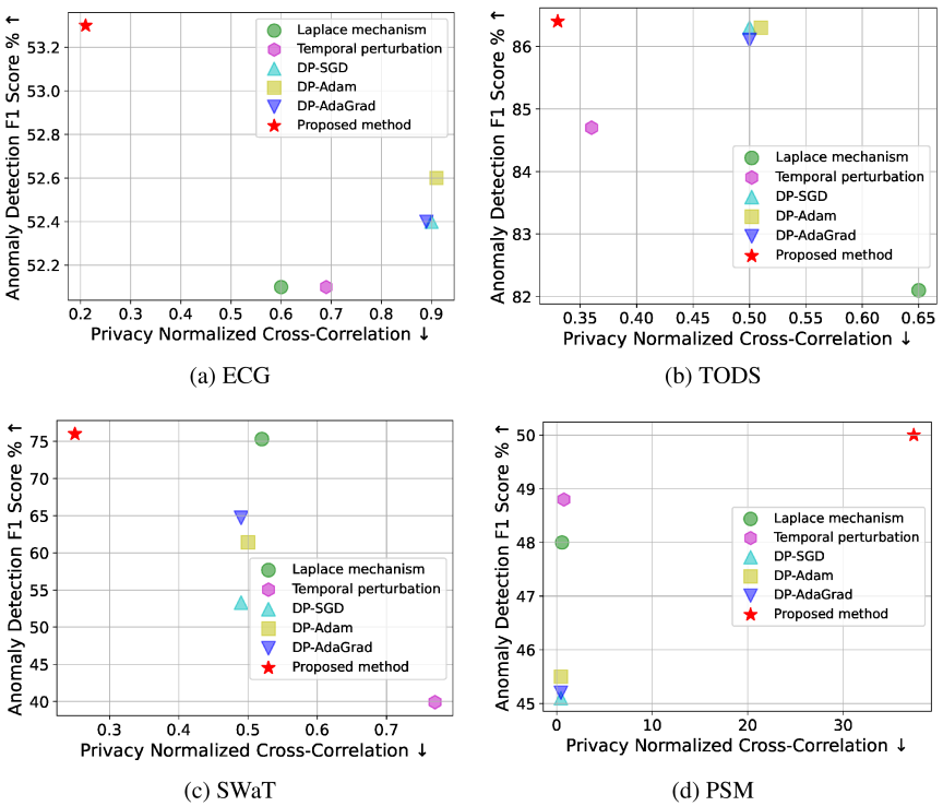
Fig. 6. Trade-off between time series similarity after anonymization and anomaly-detection performance.
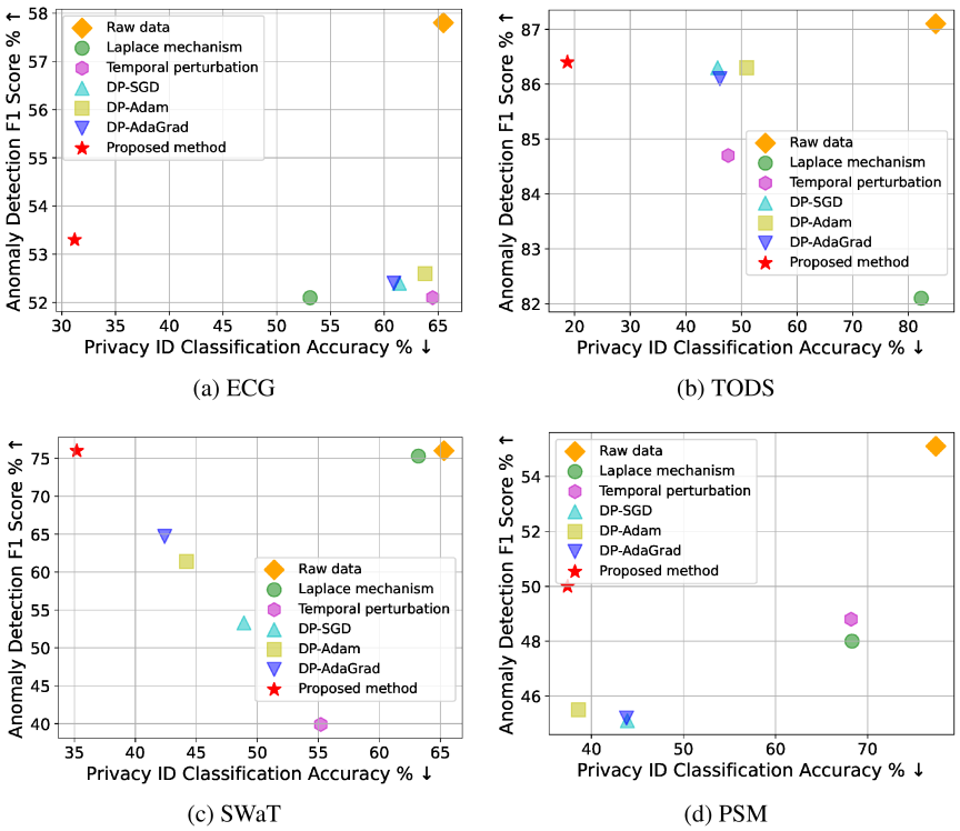
Fig. 7. Trade-off between PII removal after anonymization and anomaly-detection performance.
A.4. Standard Deviations of Experimental Results
Table 7 presents the standard deviations of the evaluation metrics reported in Table 1, computed over three experimental runs.
Appendix B. Trade-off Between Anomaly Detection and Privacy Preservation Sufficiency
Figures 6 and 7 plot the trade-off between ID-classification accuracy or similarity between pre- and post-anonymized time series (NCC) and the F1-score of anomaly detection, based on the results in Table 1. In general, there is a trade-off between anomaly-detection accuracy and privacy preservation sufficiency. However, as shown in Figs. 6 and 7, the proposed framework (\(\bigstar\)) effectively balances this trade-off, enabling strong privacy preservation while maintaining high anomaly-detection performance. Although PSM may initially appear to have a trade-off relationship, it reduces the privacy metrics significantly compared to existing anonymization methods, with only a 0.06% reduction in the F1-score for anomaly detection.
Appendix C. Effect of Noise
The noise-related parameters of the anonymization function in the proposed framework do not need to be adjusted during anonymization, whereas existing anonymization methods require tuning the amount of added noise. In Laplace mechanism, we varied the variance of the Laplace distribution used for adding noise as \(\{1, 5, 10, 100\}\). We evaluated the NCC, ID-classification accuracy, and anomaly-detection performance on SWaT using a window size of \(L=50\).
The results showed that as the amount of noise increased, NCC and ID-classification accuracy decreased, as did the anomaly-detection performance. This observation confirms the general trade-off between privacy preservation and anomaly-detection performance, as shown in Table 8. In contrast, the proposed framework successfully balances these objectives by incorporating the anonymization function.
| Anomaly detection | Privacy | ||||
| Noise | Pre | Rec | F1 (↑) | NCC (↓) | Acc (↓) |
| 1 | 99.4 | 60.6 | 75.3 | 0.52 | 63.2 |
| 5 | 76.1 | 53.8 | 63.0 | 0.23 | 50.5 |
| 10 | 20.1 | 68.8 | 53.3 | 0.18 | 31.3 |
| 100 | 12.4 | 100.0 | 22.0 | 0.13 | 2.1 |
Appendix D. Effect of Input Length
For SWaT, we evaluated NCC, ID-classification accuracy, and anomaly-detection performance by varying the window size \(L=\{50,100,150\}\). The results are summarized in Table 9.
Regardless of the window size, the proposed framework effectively reduces NCC and ID-classification accuracy, indicating strong anonymization, without significantly compromising anomaly-detection performance. Furthermore, it outperforms existing anonymization methods in both privacy preservation and anomaly-detection accuracy.
Appendix E. Scattergram of Window Vectors
In Section 5.4, we presented t-SNE visualizations of window vectors from the ECG test data. Fig. 5 compares the original data with the anonymized data produced by the proposed framework. Fig. 8 extends this analysis, illustrating the scatter plots of window vectors for all evaluated anonymization methods, including the baselines.
| Window size | 50 | 100 | 150 | ||||||||||||
| Anomaly detection | Privacy | Anomaly detection | Privacy | Anomaly detection | Privacy | ||||||||||
| Metric | Pre | Rec | F1 (↑) | NCC (↓) | Acc (↓) | Pre | Rec | F1 (↑) | NCC (↓) | Acc (↓) | Pre | Rec | F1 (↑) | NCC (↓) | Acc (↓) |
| Raw data | 99.3 | 61.2 | 76.0 | – | 65.3 | 99.8 | 58.9 | 74.1 | – | 69.6 | 99.3 | 56.6 | 73.5 | – | 67.3 |
| Laplace mechanism | 99.4 | 60.6 | 75.3 | 0.52 | 63.2 | 99.3 | 59.1 | 74.0 | 0.52 | 63.0 | 100.0 | 56.0 | 71.8 | 0.51 | 65.2 |
| Temporal perturbation | 47.9 | 60.3 | 39.9 | 0.77 | 55.2 | 87.5 | 58.1 | 69.8 | 0.76 | 64.3 | 54.7 | 61.0 | 56.0 | 0.79 | 52.0 |
| DP-SGD | 52.0 | 68.8 | 53.3 | 0.49 | 48.9 | 60.2 | 57.2 | 58.2 | 0.49 | 46.7 | 23.5 | 75.1 | 31.7 | 0.49 | 49.6 |
| DP-Adam | 63.4 | 60.6 | 61.4 | 0.50 | 44.2 | 59.3 | 56.2 | 56.9 | 0.49 | 38.7 | 63.1 | 56.5 | 53.8 | 0.49 | 41.5 |
| DP-AdaGrad | 68.4 | 62.4 | 64.7 | 0.49 | 42.4 | 46.0 | 62.8 | 44.8 | 0.49 | 44.9 | 66.3 | 61.1 | 62.0 | 0.49 | 52.2 |
| Ours | 99.4 | 61.6 | 76.0 | 0.25 | 35.2 | 99.7 | 58.8 | 74.0 | 0.13 | 26.7 | 100.0 | 58.1 | 72.1 | 0.26 | 19.9 |
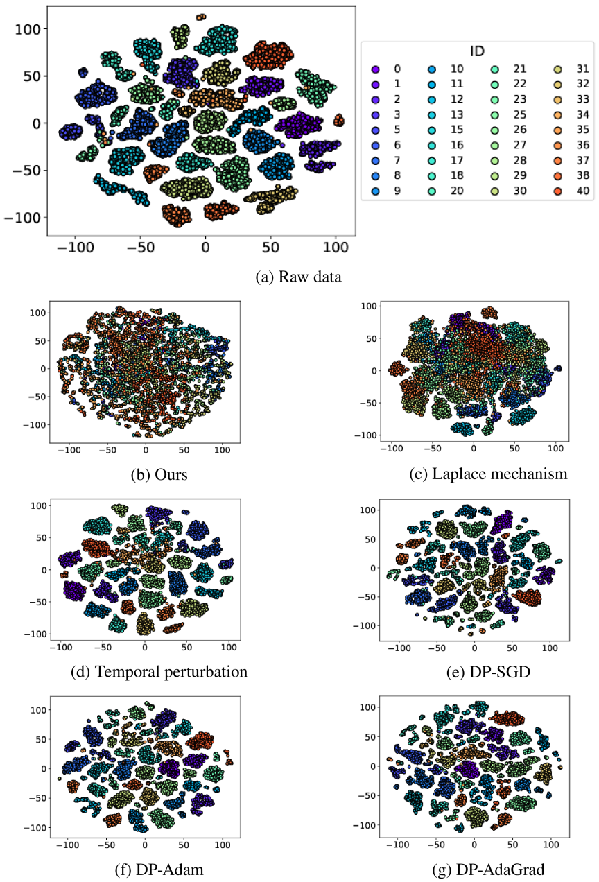
Fig. 8. Scattergram of window vectors for each anonymization method visualized using t-SNE. Existing anonymization methods often retain ID-related information, even after anonymization, resulting in clustering by ID. In contrast, the proposed framework effectively removes ID-related information through its anonymization function, leading to a more mixed distribution.
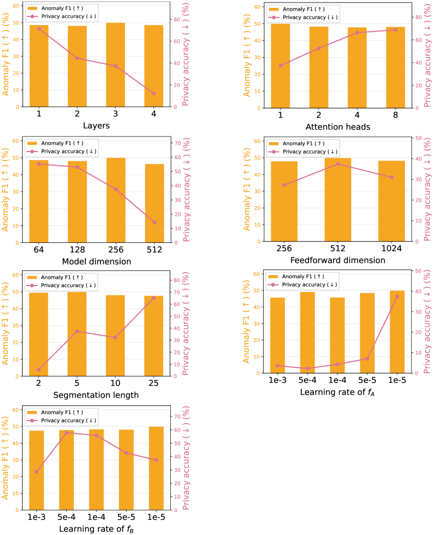
Fig. 9. Hyperparameter analysis of the proposed framework.
As shown in Fig. 8, most existing anonymization methods retain ID-related information even after anonymization. Therefore, window vectors tend to be grouped by ID, similar to that in raw data. In contrast, the proposed framework effectively removes this information through its anonymization function, visualizing window vectors as mixed and unrelated to IDs. Consequently, the ID-classification accuracy of the proposed framework is lower than that of other anonymization methods.
Appendix F. Hyperparameter Analysis
We conducted a sensitivity analysis of the hyperparameters in the proposed framework using PSM. The results obtained by varying the number of layers, number of heads, model dimensions, feed-forward dimensions, and segmentation length in \(f_A\), as well as the learning rates of \(f_A\) and \(f_B\), are shown in Fig. 9. In each subplot, the bar chart represents the anomaly-detection F1-score, and the line plot indicates the ID-classification accuracy.
Across all the hyperparameter settings, the variation in ID-classification accuracy was greater than that of the anomaly detection F1-score. In this study, we selected the hyperparameters that achieved the highest anomaly detection F1-scores. However, in practical applications, hyperparameters should be chosen by considering the trade-off between anomaly-detection performance and privacy preservation. Furthermore, because the optimal hyperparameter configuration may vary depending on dataset characteristics, careful tuning is required.
Appendix G. Contrastive Learning
Contrastive learning, a type of self-supervised learning, learns data representations by comparing data points without the need for explicit labels. Specifically, encoders are trained to map positive pairs (e.g., original and extended data) closer together and negative pairs (e.g., two data samples at different timestamps) further apart in the embedding space. We adopted contrastive learning in the time and frequency domains to generate representations of time series in \(f_B\). Several studies that applied contrastive learning to time series have generated time-based representations in the time domain 44,45,46,47,48,49,50. By generating frequency-based representations in the frequency domain, we successfully captured the behavior of time series that cannot be captured by the time component 51.
Time-based contrastive learning. Given an input window \(W_i\), we generated augmentations of \(W_i\). We used jittering, scaling, time shifts, and neighborhood segments, which are commonly used in contrastive learning, for data augmentation 42,43. For input \({W}_i\), augmented \(\hat{W}_i\) is generated and input into the contractive time encoder \(E_\mathrm{T}\). \(E_\mathrm{T}\) maps them into the time domain and obtains \(\boldsymbol{h}_i\) and \(\hat{\boldsymbol{h}}_i\) as their respective representations. \(\boldsymbol{h}_i\) (\(\boldsymbol{h}_i=E_\mathrm{T}(W_{i})\)) and \(\hat{\boldsymbol{h}}_i\) (\(\hat{\boldsymbol{h}}_i=E_\mathrm{T}(\hat{W}_{i})\)) are mapped close in the space because \(\hat{W}_i\) is generated based on \(W_i\). In contrast, representations \(\boldsymbol{h}_j\) and \(\hat{\boldsymbol{h}}_j\) of a different sample \(W_j\) and augmented \(\hat{W}_j\) are mapped away from \(\boldsymbol{h}_i\). Here, similar to 42, \((W_i, \hat{W}_i)\) is a positive pair, and \((W_i, W_j)\) and \((W_i, \hat{W}_j)\) are selected as negative pairs.
We adopted NT-Xent as the distance function (\(d\)) to minimize the similarity of positive pairs in the time domain and maximize that of negative pairs 42. In particular, the time-based contrastive loss of \(\mathcal{L}_{\mathrm{T},i}\) is defined as
Frequency-based contrastive learning. Frequency-based contrastive learning is similar to time-based contrastive learning, except that it handles Fourier-transformed input windows. Given \(W_i\), we perform a Fourier transform to obtain \(W_i^{\mathrm{F}}\). After the Fourier transform, we generate an augmented \(\hat{W}_i^{\mathrm{F}}\) using a method similar to time-based contrastive learning. \(W_i^{\mathrm{F}}\) and \(\hat{W}_i^{\mathrm{F}}\) are input into the contractive frequency encoder \(E_{\mathrm{F}}\), and their representations \(\boldsymbol{h}_i\) (\(\boldsymbol{h}_i=E _{\mathrm{F}}(W_{i})\)) and \(\hat{\boldsymbol{h}}_i\) (\(\hat{\boldsymbol{h}}_i=E_{\mathrm{F}}(\hat{W}_{i})\)) in the frequency domain are obtained. Here, \((W_i^{\mathrm{F}}, \hat{W}_i^{\mathrm{F}})\) is a positive pair and \((W_i^{\mathrm{F}}, W_j^{\mathrm{F}})\) and \((W_i^{\mathrm{F}}, \hat{W}_j^{\mathrm{F}})\) are selected as negative pairs. In particular, the frequency-based contrastive loss of \(\mathcal{L}_{\mathrm{F},i}\) is defined as
In our implementation, contrastive losses are calculated within each batch.
This article is published under a Creative Commons Attribution-NoDerivatives 4.0 Internationa License.