
Research Paper:
Boosting Cross-Domain Remaining Useful Life Prediction for Unknown Target Domain Based on Feature Decoupling
Hanchen Nan† and Chenhan Yuan
CCTEG Xi’an Research Institute (Group) Co., Ltd.
No.82, Jinye 1st Road, High-tech Industrial Development Zone, Xi’an, Shaanxi 710077, China
†Corresponding author

Remaining useful life (RUL) prediction is an important technology used to ensure safe operation of industrial equipment, which reduces maintenance costs. However, methods based on deep learning often struggle to maintain accuracy under unknown working conditions owing to the scarcity of target domain data and significant domain shifts between source and target domains. This paper proposes a novel cross-domain RUL prediction for unknown target domains based on feature decoupling, which decouples features into domain-dependent and domain-independent features. The generalizability of the model to the unknown target domain is enhanced by domain-independent features, and the performance of cross-domain RUL prediction is improved. Extensive experiments are carried out on IEEE PHM 2012 and XJTU-SY bearing datasets, and the results show that the proposed method outperformed other methods by a large margin.
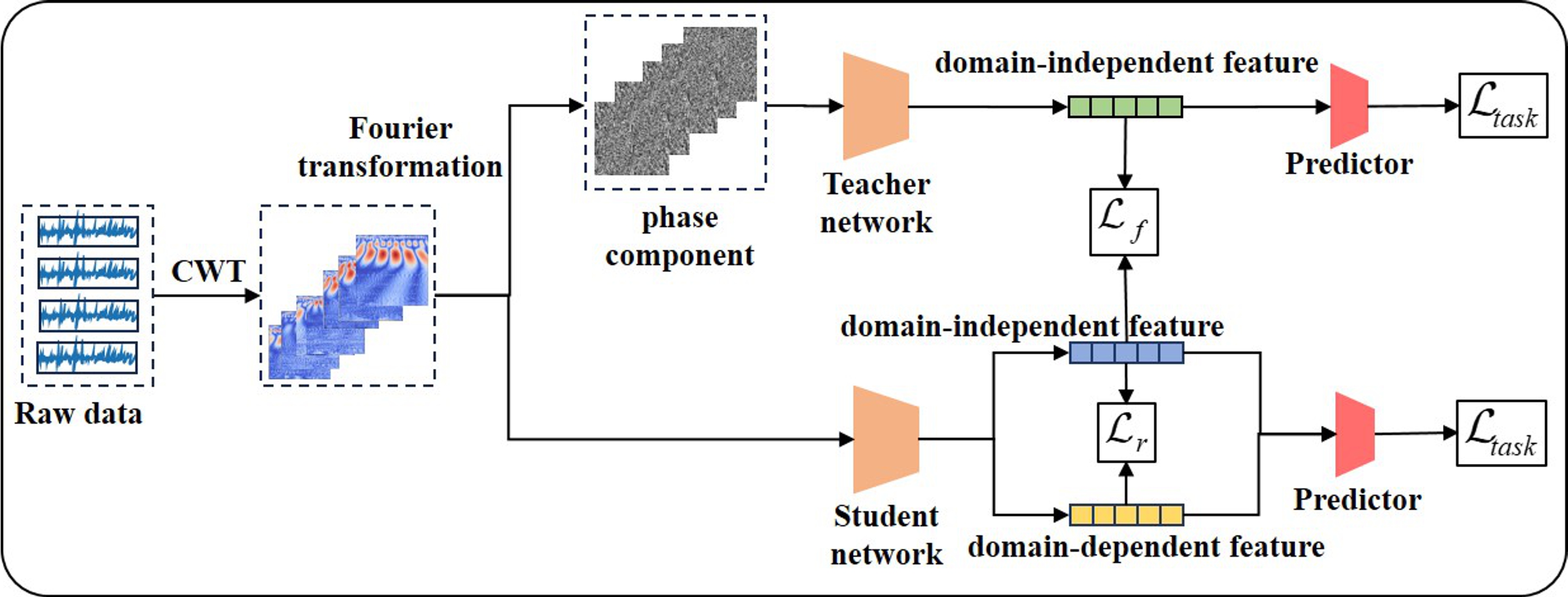
Schematic diagram of our method
1. Introduction
In the era of accelerating industrial modernization, complex equipment is extensively deployed across critical sectors such as coal mining, transportation, aerospace, and manufacturing, serving as vital infrastructure that underpins socioeconomic development. As a core task of predictive health management (PHM), equipment remaining useful life (RUL) prediction is important in ensuring safe and stable operation, reducing maintenance costs, enhancing production efficiency, and preventing catastrophic failures 1,2.
However, RUL prediction faces numerous significant challenges. The scarcity of target domain data stands out as a prominent issue. Acquiring large volumes of high-quality equipment operational data is often costly and time-consuming 3. For newly developed equipment or devices operating under special conditions, limited operational history or restricted monitoring capabilities make it difficult to accumulate sufficient historical data for constructing accurate prediction models 4. Even in domains that have accumulated data, data annotation and organization require specialized domain knowledge and substantial human resources, further limiting the effective utilization of available data 5.
Meanwhile, equipment across different domains exhibits significant differences in operational mechanisms, working environments, and failure modes 6. Traditional equipment remaining life prediction methods are typically trained on large datasets from specific domains. When existing models are applied to unknown target domains, their prediction performance significantly declines 7. Furthermore, variations in data distribution and feature spaces across domains make it challenging to directly transfer models trained in source domains to unknown target domains, further complicating cross-domain equipment remaining life prediction.
In recent years, with extensive research on methods such as transfer learning and domain generalization 8, the performance of cross-domain equipment lifetime prediction has significantly improved 9. Existing studies primarily focus on the following directions: First, feature alignment techniques based on adversarial learning, which narrow the gap between different domain data distributions through adversarial training to improve the generalization capability of the model in the target domain 10,11,12; Second, some methods try to enhance the transferable useful knowledge acquired from source domains through meta-learning to enable rapid adaptation to new domains 13,14. Third, other methods integrate techniques such as few-shot and self-supervised learning to reduce overfitting to labeled data 15,16. However, most of these approaches focus on learning the overall feature distribution of the source domain, failing to deeply explore the inherent transfer potential of different feature types (e.g., domain-relevant and domain-irrelevant features) within equipment operational data. This results in insufficient generalization performance during cross-domain applications. To address these challenges, some studies have explored feature decoupling methods. These approaches aim to enhance domain adaptability by explicitly distinguishing domain-relevant and irrelevant information at the feature level. Nevertheless, their performance in complex industrial applications remains limited, calling for further research.
To address this challenge, this paper proposes a novel cross-domain RUL prediction method towards unknown domains based on a feature decoupling strategy. The proposed method decomposes features into domain-dependent and domain-independent components. Domain-dependent features relate to equipment type and operating conditions, while domain-independent features exhibit consistent distribution across domains. Given the inherent domain differences between source and target domains, the core challenge lies in accurately extracting these domain-independent features. Specifically, the method first preprocesses raw time-series data using continuous wavelet transform (CWT). Then, the data is further converted into amplitude and phase components. Based on knowledge distillation, a teacher-student network architecture is constructed. The teacher network, fed with the phase components, specializes in extracting domain-independent features, while the student network processes the wavelet-transformed data. Guided by the teacher network, the student network extracts domain-dependent and domain-independent features, which enables accurate RUL prediction. Domain-independent features are defined as those that capture degradation semantics invariant across operating conditions, which exhibit consistent statistical properties across domains. Domain-dependent features are defined as those encoding domain-specific factors such as rotational speed, load, or sensor characteristics, which vary significantly between source and target domains.
The contributions of this paper are summarized as follows:
-
1.
This paper proposes a novel cross-domain RUL prediction based on feature disentanglement towards unseen target domains. Domain-related and domain-independent features are extracted to improve the generalizability of the model to unknown target domains.
-
2.
A teacher-student collaborative knowledge distillation framework is constructed. The teacher network learns domain-independent features based on frequency learning and guides the student network to learn domain-related features through knowledge distillation.
-
3.
Experiments on multiple tasks demonstrate the superiority of the method over other methods.
2. Related Work
RUL prediction is a central focus in PHM research, aiming to estimate the time until a system or component fails under current operating conditions. Traditional approaches to RUL estimation can be broadly categorized into model-based, data-driven, and hybrid methods 17. Model-based techniques rely on physical degradation models derived from domain knowledge. While physically interpretable, these methods often require precise system modeling and may not generalize well under uncertain or complex operating environments. In contrast, data-driven approaches leverage historical sensor data and statistical or machine learning models to infer degradation patterns. Early efforts employed stochastic processes like Wiener or Gamma processes to model degradation trajectories 18. More recently, deep learning architectures, particularly recurrent neural networks, long short-term memory (LSTM) networks, and convolutional neural networks (CNNs), have demonstrated strong performance in capturing temporal dependencies and nonlinear degradation dynamics. He et al. 19 proposed a dual-correlation adaptive gated graph convolutional network for bearing RUL prediction by creating a predefined double correlation graph and an adaptive graph. Qi et al. 20 proposed a multi-task graph isomorphism network with an attention mechanism, introducing a parameter-sharing mechanism and self-attention mechanism for simultaneous fault diagnosis and RUL prediction. Zhang et al. 21 presented a local enhanced channel self-attention based on a Transformer method to capture the long-term dependencies; then Transformer architecture was compared with RNN/CNN-based methods. Gandhudi and Gangadharan 22 proposed a quantum neural network to facilitate an effective trade-off between convergence speed and model generalization by adaptively adjusting the learning rate throughout training optimized through quantum annealing.
Beyond conventional within-domain modeling, cross-domain RUL prediction has been employed to address data scarcity and distribution shifts across different operational conditions, equipment variants, or fault modes. Transfer-learning and domain-adaptation techniques enable knowledge transfer from source domains with abundant labeled data to target domains with limited or unlabeled data. Nejjar et al. 23 presented an adversarial domain-adaptation method for cross-domain RUL prediction considering the different phases of the operation profiles separately; they aligned the marginal distributions of each phase of the operation profile in the source-domain with its counterpart in the target-domain. To address the scenarios of few-shot and cross-domain conditions in RUL prediction, Yang and Wang 24 proposed a meta-learning with deep flow kernel network model that learns kernel features in a data-driven manner and considers them as latent variables to improve the performance. Liu et al. 25 presented a RUL transfer prediction method using a multi-scale subsequence alignment to select the most informative source-domain subsequences and an interpretable transfer-learning model to embed a self-attention mechanism and a Bayesian linear layer into the domain-adaptation. These cross-domain strategies significantly improve model generalizability and reduce the need for extensive retraining, making them valuable in industrial applications where labeled failure data are costly or impractical to obtain. Tian et al. 26 proposed an uncertainty-weighted with gradient-based to upweighted domain generalization (UWGRDG) method including a dual-teacher knowledge distillation framework based on adversarial learning to capture two more fine-grained internally invariant features between different domains for RUL prediction under unseen conditions. Zhang et al. 27 proposed a joint domain-adaptive Transformer (JDATransformer) method and constructed global feature distribution alignment within the Transformer to improve the performance of cross-domain RUL prediction. Li et al. 28 proposed a domain-invariant and consistent ordinal representation learning method using maximum mean discrepancy to align the feature distributions of different source-domain and alleviate the overfitting problem of the model in given domains.
However, current methods are unable to effectively utilize limited source-domain data, and there is room for improvement in terms of model generalization to unknown domains. The method proposed in this paper fully accounts for the multidimensional distribution characteristics of data and can adapt to RUL prediction from unknown domains.
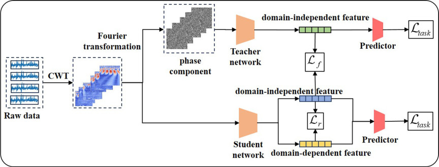
Fig. 1. Schematic diagram of our method.
3. Methods
The challenge in cross-domain RUL prediction for unknown target domains lies in the limited training data, coupled with domain differences between source and target domains. Since the target domain is not known in advance, the prediction model must adapt to diverse target domains. Therefore, this approach decouples features into domain-independent and domain-dependent components, leveraging domain-independent features to enhance generalization capabilities across unknown target domains. A schematic representation of this method is shown in Fig. 1.
3.1. Data Preprocessing
CWT is a multiscale analysis method capable of simultaneously capturing frequency-domain and time-domain features. It maps raw one-dimensional time-series data into a two-dimensional time-frequency feature representation, revealing local dynamic characteristics and transient changes. CWT is expressed as
3.2. Domain-Invariant Feature Extraction
After undergoing Fourier transformation, the phase component of the data contains more high-level semantic information, representing the content features of the data with minimal association to the domain 29,30. In contrast, the amplitude component primarily contains low-level statistical information, which is significantly influenced by the domain. Therefore, the proposed method extracts domain-independent features based on the phase component of the data. For the input data \(x\), applying the Fourier transform yields the following representation:
3.3. Feature Extraction Based on Knowledge Distillation
To further extract and use domain-agnostic features in frequency domain, a feature-extraction strategy using knowledge distillation is introduced 31,32,33. The teacher network first takes the phase component \(P(x)\) as input and then extracts high-level discriminative features through the feature extractor \(F^T\) and predictor \(P^T\), and is trained using the prediction loss \(L_{\mathit{task}}\) to optimize prediction performance:
The features extracted by the student network are decomposed into domain-dependent features \(F_r^S(x_i)\) and domain-independent features \(F_i^S(x_i)\). Therefore, a feature loss \(L_f\) is introduced between these domain-independent features and those extracted by the teacher network, encouraging the student network to emulate the discriminative capability of the teacher network in feature learning:
When decoupling features extracted from student networks into domain-dependent and domain-independent components, their correlation should be minimized to enhance their distinctiveness. A feature correlation loss is introduced,
The overall loss function of the student network is
4. Results and discussion
4.1. Datasets
IEEE PHM 2012 Rolling Bearing Dataset 34 and the XJTU-SY dataset 35 were used in this study. The IEEE PHM 2012 Rolling Bearing Dataset was obtained from the PRONOSTIA platform and contains lifetime data of 17 bearings under three operating conditions, covering multiple failure modes, reflecting the diversity of degradation behavior. The XJTU-SY dataset is a full-lifetime degradation-analysis dataset used for testing lifetime modeling and prediction. It contains 15 complete databases of vibration signals from degradation to failure. The two datasets comprise multiple sub-datasets collected under varying rotational speeds and pressures, with relevant details in Table 1.
| Datasets |
Speeds [rpm] |
Pressures [kN] |
Subdatasets |
| XJTU-SY | 2100 | 12 | 1-1–1-5 |
| 2250 | 11 | 2-1–2-5 | |
| 2400 | 10 | 3-1–3-5 | |
| IEEE PHM 2012 | 1800 | 4000 | 1-1–1-7 |
| 1650 | 4200 | 2-1–2-7 | |
| 1500 | 5000 | 3-1–3-3 |
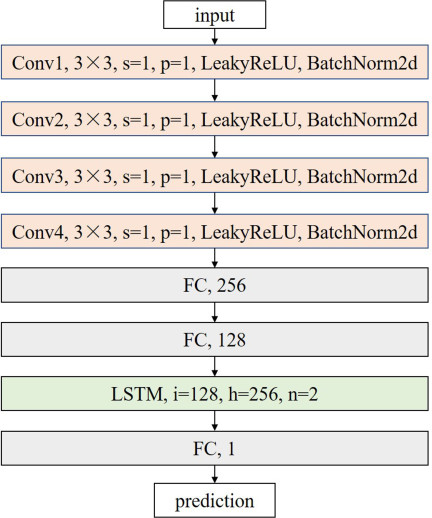
Fig. 2. Architectures of teacher and student networks.
4.2. Experimental Setting
In our experiments, one subset was selected as the source domain and another as the target domain to set up different cross-domain RUL prediction tasks. For each task, the dataset was divided into training and testing sets at a ratio of \(8:2\). To evaluate the accuracy of our method, two commonly used performance metrics were employed: mean absolute error (MAE) and root mean squared error (RMSE). All experiments were conducted under a standardized environment. To ensure robustness of the results, each cross-domain task was randomly repeated 10 times, with the average RMSE and MAE serving as the final evaluation metrics. The model with the same architecture as the student network and trained only by \(L_{\mathit{task}}\) was used as the baseline.
In this study, the teacher and student networks had the same architecture that consisted of three core components: a feature extractor, feature bottleneck network, and predictor, as shown in Fig. 2. The feature extractor comprised four stacked 2D convolutional layers (Conv2d), each employing a \(3 \times 3\) kernel with stride 1 and a padding of 1 to preserve spatial resolution. Following each convolution, a LeakyReLU activation function introduced nonlinearity, while a BatchNorm2d layer stabilized training and accelerates convergence. The feature bottleneck network served as an intermediate representation adapter, primarily facilitating knowledge distillation between the teacher and student networks. It consisted of two fully connected layers that projected the high-dimensional feature maps from the extractor into a lower-dimensional embedding space. The predictor was implemented as an LSTM network, which took the bottleneck-processed features as input, with configurable parameters including input feature dimension, hidden state size, and number of stacked layers. The final RUL estimate was produced by a linear fully connected layer with a single output neuron, ensuring direct regression to the remaining life value.
All experiments were conducted in a standardized environment; the details of the parameter settings of the experiments are listed in Table 2.
| Parameter | Value |
| Learning rate | 0.0001 |
| Batch size | 16 |
| Optimizer | Adam |
| \(\alpha\) | 3 |
| \(\beta\) | 0.1 |
| Epoch | 50 |
| Task | Source | Target | Baseline | Ours |
| T1-1-1 | 1-1 | 1-2 | 0.427\(\pm\)0.0782 | 0.337\(\pm\)0.0018 |
| T1-1-2 | 1-1 | 2-2 | 0.413\(\pm\)0.0077 | 0.276\(\pm\)0.0312 |
| T1-1-3 | 1-1 | 3-2 | 0.345\(\pm\)0.0137 | 0.299\(\pm\)0.0097 |
| T1-2-1 | 1-2 | 1-1 | 0.345\(\pm\)0.1002 | 0.199\(\pm\)0.0208 |
| T1-2-2 | 1-2 | 2-2 | 0.275\(\pm\)0.0089 | 0.200\(\pm\)0.0032 |
| T1-2-3 | 1-2 | 3-1 | 0.362\(\pm\)0.0166 | 0.280\(\pm\)0.0117 |
| T2-1-1 | 2-1 | 1-1 | 0.324\(\pm\)0.0036 | 0.212\(\pm\)0.0031 |
| T2-1-2 | 2-1 | 1-2 | 0.334\(\pm\)0.0239 | 0.299\(\pm\)0.0329 |
| T2-1-3 | 2-1 | 3-1 | 0.409\(\pm\)0.0015 | 0.228\(\pm\)0.0052 |
| T2-2-1 | 2-2 | 1-1 | 0.271\(\pm\)0.0240 | 0.288\(\pm\)0.0131 |
| T2-2-2 | 2-2 | 3-1 | 0.268\(\pm\)0.0124 | 0.195\(\pm\)0.0117 |
| T2-2-3 | 2-2 | 3-2 | 0.268\(\pm\)0.0058 | 0.228\(\pm\)0.0093 |
| T3-1-1 | 3-1 | 1-2 | 0.398\(\pm\)0.0247 | 0.285\(\pm\)0.0145 |
| T3-1-2 | 3-1 | 2-1 | 0.231\(\pm\)0.0336 | 0.291\(\pm\)0.0279 |
| T3-1-3 | 3-1 | 2-2 | 0.295\(\pm\)0.0028 | 0.158 \(\pm\)0.0019 |
| T3-2-1 | 3-2 | 1-2 | 0.474\(\pm\)0.0457 | 0.409\(\pm\)0.0289 |
| T3-2-2 | 3-2 | 2-1 | 0.446\(\pm\)0.0109 | 0.374\(\pm\)0.0032 |
| T3-2-3 | 3-2 | 3-1 | 0.268\(\pm\)0.0163 | 0.377\(\pm\)0.0165 |
| Average | 0.328\(\pm\)0.0182 | 0.274\(\pm\)0.0179 | ||
4.3. Results and Analysis
Table 3 shows the experimental results on the IEEE PHM 2012 dataset. The results demonstrate that when significant operational condition differences exist between the source and target domains, our method reduces the average MAE for all cross-domain RUL prediction tasks from 0.328 for the baseline method to 0.274, representing a 16.46% decrease. This indicates the model can identify and adapt to degradation patterns under different operational conditions. For task T3-1-3, our method reduces MAE from 0.295 of the baseline method to 0.158, achieving a substantial 46.44% decrease. This further validates the robustness and adaptability of the model in handling complex variations in operating conditions.
| Task | Source | Target | Baseline | Ours |
| S1-1-1 | 1-1 | 1-2 | 0.274\(\pm\)0.0431 | 0.248\(\pm\)0.0152 |
| S1-1-2 | 1-1 | 2-2 | 0.261\(\pm\)0.0603 | 0.214\(\pm\)0.0414 |
| S1-1-3 | 1-1 | 3-2 | 0.304\(\pm\)0.0363 | 0.270\(\pm\)0.0143 |
| S1-2-1 | 1-2 | 1-1 | 0.267\(\pm\)0.0095 | 0.259\(\pm\)0.0008 |
| S1-2-2 | 1-2 | 2-2 | 0.375\(\pm\)0.0578 | 0.266\(\pm\)0.0244 |
| S1-2-3 | 1-2 | 3-1 | 0.259\(\pm\)0.0746 | 0.247\(\pm\)0.0098 |
| S2-1-1 | 2-1 | 1-1 | 0.332\(\pm\)0.0075 | 0.319\(\pm\)0.0032 |
| S2-1-2 | 2-1 | 1-2 | 0.364\(\pm\)0.0546 | 0.325\(\pm\)0.0076 |
| S2-1-3 | 2-1 | 3-1 | 0.315\(\pm\)0.0324 | 0.294\(\pm\)0.0056 |
| S2-2-1 | 2-2 | 1-1 | 0.297\(\pm\)0.0622 | 0.346\(\pm\)0.0262 |
| S2-2-2 | 2-2 | 3-1 | 0.333\(\pm\)0.0090 | 0.267\(\pm\)0.0046 |
| S2-2-3 | 2-2 | 3-2 | 0.327\(\pm\)0.0363 | 0.255\(\pm\)0.0164 |
| S3-1-1 | 3-1 | 1-2 | 0.282\(\pm\)0.0095 | 0.246\(\pm\)0.0042 |
| S3-1-2 | 3-1 | 2-1 | 0.286\(\pm\)0.0359 | 0.305\(\pm\)0.0278 |
| S3-1-3 | 3-1 | 2-2 | 0.271\(\pm\)0.0687 | 0.259\(\pm\)0.0324 |
| S3-2-1 | 3-2 | 1-2 | 0.286\(\pm\)0.0032 | 0.243\(\pm\)0.0012 |
| S3-2-2 | 3-2 | 2-1 | 0.437\(\pm\)0.0253 | 0.319\(\pm\)0.0146 |
| S3-2-3 | 3-2 | 3-1 | 0.368\(\pm\)0.0468 | 0.261\(\pm\)0.0248 |
| Average | 0.309\(\pm\)0.0955 | 0.275\(\pm\)0.0212 | ||
Experimental results on the XJTU-SY dataset are shown in Table 4. When vertical and horizontal composite load differences exist between source and target domains, our method can reduce the average MAE from 0.309 of the baseline method to 0.275 across all tasks, representing an 11% error reduction. This indicates the model effectively captures degradation evolution patterns under composite stresses. Under optimal conditions, the proposed method reduces MAE on task S3-2-3 from 0.368 of the baseline method to 0.261, a 29.08% decrease. The proposed method maintains strong performance even in challenging transfer tasks under extreme operating conditions. For instance, in task S3-2-2, significant differences in rotational speed and pressure were observed.
| Methods | IEEE PHM 2012 | XJTU-SY | Average | |||
| RMSE | MAE | RMSE | MAE | RMSE | MAE | |
| CNN | 0.387\(\pm\)0.0472 | 0.309\(\pm\)0.0245 | 0.378\(\pm\)0.0356 | 0.302\(\pm\)0.0885 | 0.383\(\pm\)0.0431 | 0.306\(\pm\)0.0575 |
| Mixup | 0.357\(\pm\)0.0886 | 0.285\(\pm\)0.0479 | 0.381\(\pm\)0.0932 | 0.304\(\pm\)0.0577 | 0.369\(\pm\)0.0903 | 0.295\(\pm\)0.0532 |
| MPML | 0.364\(\pm\)0.0443 | 0.296\(\pm\)0.0569 | 0.386\(\pm\)0.0432 | 0.302\(\pm\)0.0146 | 0.375\(\pm\)0.0402 | 0.299\(\pm\)0.0334 |
| CORAL | 0.357\(\pm\)0.0125 | 0.285\(\pm\)0.0466 | 0.385\(\pm\)0.0554 | 0.307\(\pm\)0.0453 | 0.371\(\pm\)0.0380 | 0.296\(\pm\)0.0459 |
| DWDAN | 0.349\(\pm\)0.0366 | 0.290\(\pm\)0.0478 | 0.362\(\pm\)0.0568 | 0.292\(\pm\)0.0266 | 0.356\(\pm\)0.0454 | 0.291\(\pm\)0.0347 |
| MMD | 0.459\(\pm\)0.0443 | 0.366\(\pm\)0.0570 | 0.377\(\pm\)0.0488 | 0.301\(\pm\)0.0365 | 0.418\(\pm\)0.0419 | 0.333\(\pm\)0.0438 |
| DANN | 0.350\(\pm\)0.0135 | 0.279\(\pm\)0.0557 | 0.372\(\pm\)0.0445 | 0.297\(\pm\)0.0397 | 0.361\(\pm\)0.0284 | 0.288\(\pm\)0.0506 |
| GroupDRO | 0.377\(\pm\)0.0993 | 0.301\(\pm\)0.0444 | 0.391\(\pm\)0.0532 | 0.312\(\pm\)0.0499 | 0.384\(\pm\)0.0678 | 0.307\(\pm\)0.0467 |
| RSC | 0.359\(\pm\)0.0775 | 0.287\(\pm\)0.0634 | 0.366\(\pm\)0.0688 | 0.292\(\pm\)0.0699 | 0.363\(\pm\)0.0757 | 0.289\(\pm\)0.0657 |
| JDATransformer | 0.351\(\pm\)0.0347 | 0.285\(\pm\)0.0578 | 0.354\(\pm\)0.0433 | 0.280\(\pm\)0.0478 | 0.353\(\pm\)0.0403 | 0.283\(\pm\)0.0495 |
| Ours | 0.343\(\pm\)0.0201 | 0.274\(\pm\)0.0179 | 0.344\(\pm\)0.0183 | 0.275\(\pm\)0.0212 | 0.344\(\pm\)0.0195 | 0.275\(\pm\)0.0187 |
4.4. Comparison with Other Methods
To comprehensively evaluate the performance of the proposed method, we conducted comparative analyses with multiple approaches, including traditional CNNs, domain-adversarial neural networks (DANN) 36, data augmentation mixup 37, multi-task pointwise mutual information learning (MPML) 38, covariance alignment (CORAL) 39, domain weighted distribution adaptation network (DWDAN) 40, maximum mean discrepancy (MMD) 41, GroupDRO 42, and representation self-challenging (RSC) 43, JDATransformer 27.
As shown in Table 5, the proposed method obtains the optimal performance, demonstrating significantly enhanced generalization capabilities, particularly under data scarcity and high interdomain variability. On the IEEE PHM 2012 dataset, the proposed method reduces RMSE by approximately 25.3% compared with the worst-performing MMD method and improves MAE by 9.0% over GroupDRO. On the XJTU-SY dataset, the proposed method achieves an RMSE improvement of approximately 8.8% over MMD and a MAE improvement of 11.9% over GroupDRO. From the results, GroupDRO exhibits overfitting to the source domain during training, leading to poor generalization on the target domain. GroupDRO aggressively upweights difficult source groups, which in this case correspond to bearings with atypical degradation patterns. These results demonstrate that our method obtains significantly better overall performance compared to other methods.
4.5. Discussion
The experimental results presented in Table 5 demonstrate a clear and consistent performance advantage of the proposed method across both benchmark datasets under realistic domain shift conditions that simulate variations in operating speed, load, and data acquisition environments. Our method achieves the lowest average MAE and RMSE of all compared methods, outperforming not only conventional deep learning models but also state-of-the-art domain generalization techniques such as GroupDRO, MMD, DANN, and JDATransformer by statistically significant margins. This consistent superiority underscores the robustness and transferability of our framework, particularly in practical industrial settings where labeled target data is unavailable and operational conditions are inherently non-stationary.
The CNN trained solely with task loss performs poorly, as it lacks mechanisms to mitigate distributional discrepancies across domains. Data augmentation strategies like Mixup and meta-learning approaches such as MPML yielded modest gains but remained fundamentally constrained by their reliance on source-domain statistics, limiting their ability to extrapolate to unseen conditions. Similarly, distribution alignment methods, including CORAL and DWDAN, attempted to match marginal or conditional feature distributions across domains. However, they often failed to enforce invariance at the semantic level of degradation progression, leading to suboptimal generalization. Domain-adversarial methods like DANN and domain-gap reducing methods like MMD, while theoretically appealing, suffer training instability, particularly due to conflicting gradient dynamics in the adversarial game, and tend to produce collapsed or overly smoothed representations when source domains exhibit high heterogeneity, as is common in real-world machinery data. Notably, GroupDRO exhibited unexpectedly poor performance on the XJTU-SY dataset, underperforming even simple baselines. Further analysis reveals that this stems from its tendency to overfit to minority or atypical source groups during worst-case risk minimization. In this context, bearings with anomalous or nonrepresentative degradation trajectories were aggressively upweighted, causing the model to neglect more generalizable patterns and catastrophically fail on the target domain. While JDATransformer represents the current state-of-the-art method by leveraging transformer-based attention to align cross-domain temporal dynamics, our method surpassed it by grounding representation learning in physics-informed signal priors by decomposing vibration signals via the CWT and using the phase component as a stable, domain-invariant supervisory signal. This integration of domain knowledge with structured disentanglement enables the model to isolate degradation semantics from confounding operational factors, resulting in more meaningful, interpretable, and transferable features. These results validate that combining signal processing fundamentals with modern representation learning offers a more principled and effective pathway to robust RUL prediction than purely data-driven or distribution-centric domain generalization strategies.
4.6. Ablation Studies
We constructed three loss functions and conducted ablation studies to analyze their impact on performance; the results are shown in Table 6. We evaluated the contribution of each module to model performance improvement by comparing MAE across different loss-function combinations.
First, when using only the prediction loss, the average MAE on the IEEE PHM 2012 and XJTU-SY datasets was 0.328 and 0.309, respectively, an average of 0.319. This indicates that prediction accuracy without the assistance of additional loss functions has certain limitations. After incorporating feature loss, model performance significantly improved: MAE decreased to 0.292 on the IEEE PHM 2012 dataset and 0.298 on the XJTU-SY dataset. This demonstrates that the distillation module effectively transfers knowledge from the teacher network to the student network, enhancing the ability of the model to extract key features, improving prediction accuracy. Further incorporating the correlation loss function reduced MAE on the IEEE PHM 2012 dataset to 0.274 and on the XJTU-SY dataset to 0.275. This demonstrates that correlation loss can improve the generalizability and prediction accuracy of the model.
| Loss | IEEE PHM 2012 | XJTU-SY |
| \(L_{\mathit{task}}\) | 0.328\(\pm\)0.0182 | 0.309\(\pm\)0.0955 |
| \(L_{\mathit{task}}+L_{f}\) | 0.292\(\pm\)0.0088 | 0.298\(\pm\)0.0221 |
| \(L_{\mathit{task}}+L_{f}+L_{r}\) | 0.274\(\pm\)0.0179 | 0.275\(\pm\)0.0212 |
4.7. Efficiency and Real-Time Feasibility
To assess practical applicability in time-sensitive settings, we measured the average inference time for all compared methods. The hardware platform included Intel® Xeon® Silver 4214R CPU and NVIDIA RTX 3080 Ti GPU. The results are shown in Table 7. For Mixup, MPML, CORAL, DWDAN, MMD, DANN, GroupDRO, RSC, and our proposed method, the same architectures were used as the backbone; thus, they obtained similar inference time. However, for the transformer-based method, JDATransformer, the inference time was significantly extended. The moderate overhead of our method stems primarily from the LSTM predictor and feature bottleneck computation, but remains well within the tolerance for real-time monitoring, especially considering that bearing vibration data is typically acquired at sampling intervals of tens to hundreds of milliseconds.
| Method |
Inference time [ms] |
Method |
Inference time [ms] |
| CNN | 6.2 | Mixup | 8.5 |
| MPML | 9.1 | CORAL | 8.5 |
| DWDAN | 8.6 | MMD | 8.5 |
| DANN | 8.5 | GroupDRO | 8.5 |
| RSC | 8.7 | JDATransformer | 24.3 |
| Ours | 8.5 |
4.8. Hyperparameter Tuning
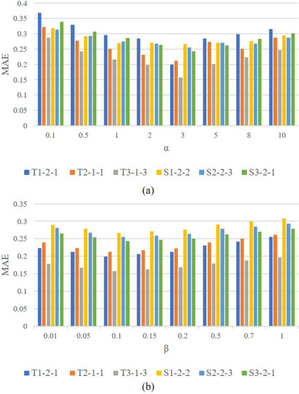
Fig. 3. Performance of different hyperparameters.
Equation (7) contains two hyperparameters \(\alpha\) and \(\beta\). We experimentally investigate their impact on model performance. \(\alpha\) was used to adjust the weight of the feature correlation loss; the experimental results are shown in Fig. 3(a). As \(\alpha\) increases from 0.1 to 3, MAE continuously decreases on multiple tasks, indicating sustained performance improvement. This demonstrates that appropriately strengthening discriminative features benefits model generalization. The model achieves optimal overall performance with the lowest average MAE when \(\alpha=3\). However, further increasing \(\alpha\) leads to performance regression on some tasks due to overly strong feature correlation loss interfering with the model’s learning of the primary task.
The weight \(\beta\), which is used to measure feature loss is illustrated in Fig. 3(b). As \(\beta\) increased from 0.01 to 0.1, the model performance is continuously optimized, with MAE reaching its lowest values on T1-2-1 and T3-1-3. This demonstrates that moderately reinforcing feature consistency enhances cross-domain robustness. The overall error is minimized at \(\beta=0.1\), validating the effectiveness of the feature consistency mechanism. However, when \(\beta\) exceeds 0.15, model performance slightly declined. This may stem from an overly weakened ability to model domain differences between teacher and student features, leading to overfitting to the source domain feature distribution. When \(\beta=1\), errors across all tasks generally increase, further demonstrating that excessively large values suppress the model’s learning of target domain-specific information.
In the experiments, when studying one hyperparameter, the other hyperparameters were kept constant. When studying \(\alpha\), \(\beta\) was fixed at 0.1; when studying \(\beta\), \(\alpha\) was fixed at 3.0. The model achieved its best overall MAE when \(\alpha=3\) and \(\beta=0.1\), as determined by the two-stage grid search over the hyperparameter space.
5. Conclusions
This paper addresses the challenges of data scarcity and domain differences in unknown target domains for RUL prediction. We propose a cross-domain RUL prediction method for unknown target domains. By introducing frequency-domain phase information and a feature decoupling mechanism, this method effectively separates domain-relevant and domain-irrelevant features. Multiple generalization tasks were designed. Experimental results demonstrate performance superior to that of existing mainstream methods on both the IEEE PHM 2012 and XJTU-SY datasets, while maintaining stable prediction capabilities under data perturbations and drastic domain- distribution variations.
Limitations and future work. The proposed method assumes access to fully labeled source-domain data from known operating conditions. It may be impractical in many industrial settings where labeling RUL is costly, time-consuming, or even infeasible owing to long equipment lifespans. This dependency on annotated source data limits scalability in low-resource scenarios. In the future, we will investigate semi-supervised, self-supervised, or weakly supervised variants of the framework to reduce annotation burden while preserving generalization capability.
The proposed method was evaluated on bearing prognostics, which represents only one class of mechanical components. While bearings are a canonical testbed in prognostics research, real-world industrial systems involve diverse assets. A limitation of this work is the lack of validation across broader machinery types and application domains. In the future, we will focus on extending and evaluating the framework on multicomponent and cross-system datasets to assess its generalizability beyond bearing health monitoring.
- [1] B. Zhang, N. Li, J. Huang, T. Arakawa, K. Ishii, and R. Yashima, “Remaining useful life prediction for tools based on monitoring data and stochastic degradation model,” J. Adv. Comput. Intell. Intell. Inform., Vol.29, No.3, pp. 668-676, 2025. https://doi.org/10.20965/jaciii.2025.p0668
- [2] J. Zhao, D. He, Z. Jin, X. Zhang, and J. Zhou, “A new method for bearing remaining useful life prediction based on dynamic wavelet and physical information constraints,” Expert Systems with Applications, Vol.296, Article No.129023, 2026. https://doi.org/10.1016/j.eswa.2025.129023
- [3] J. Han, Y. Kwon, and H. Yoon, “Mamba-attention: A self-supervised framework for efficient remaining useful life prediction,” Reliability Engineering and System Safety, Vol.265, Article No.111492, 2026. https://doi.org/10.1016/j.ress.2025.111492
- [4] S. O. Khairunnisa, Z. Chen, and M. Komachi, “Improving domain-specific ner in the indonesian language through domain transfer and data augmentation,” J. Adv. Comput. Intell. Intell. Inform., Vol.28, No.6, pp. 1299-1312, 2024. https://doi.org/10.20965/jaciii.2024.p1299
- [5] H. Shao, D. Jing, N. Xia, Z. Tang, and D. Zhong, “Universal domain adaptation in intelligent fault diagnosis via simulating unseen classes,” IEEE Trans. on Automation Science and Engineering, Vol.22, pp. 9178-9189, 2025. https://doi.org/10.1109/tase.2024.3502426
- [6] T. Hu, Z. Mo, and Z. Zhang, “Neural ode powered model for bearing remaining useful life predictions with intra- and inter-domain shifts,” Advanced Engineering Informatics, Vol.64, Article No.103077, 2025. https://doi.org/10.1016/j.aei.2024.103077
- [7] I. Barry and M. Hafsi, “Advanced multi-model prediction of aircraft engine remaining useful life with random sampling-based class balancing and voting-based features selection,” Engineering Applications of Artificial Intelligence, Vol.156, Article No.111201, 2025. https://doi.org/10.1016/j.engappai.2025.111201
- [8] A. R. A. Besari, F. Ardilla, A. A. Saputra, Kurnianingsih, T. Obo, and N. Kubota, “Egocentric behavior analysis based on object relationship extraction with graph transfer learning for cognitive rehabilitation support,” J. Adv. Comput. Intell. Intell. Inform., Vol.29, No.1, pp. 12-22, 2025. https://doi.org/10.20965/jaciii.2025.p0012
- [9] X. Lei, H. Shao, Z. Tang, S. Xu, and D. Zhong, “Cross-domain remaining useful life prediction under unseen condition via mixed data and domain generalization,” Measurement, Vol.244, Article No.116451, 2025. https://doi.org/10.1016/j.measurement.2024.116451
- [10] J. Shang, D. Xu, M. Li, H. Qiu, C. Jiang, and L. Gao, “Remaining useful life prediction of rotating equipment under multiple operating conditions via multi-source adversarial distillation domain adaptation,” Reliability Engineering and System Safety, Vol.256, Article No.110769, 2025. https://doi.org/10.1016/j.ress.2024.110769
- [11] Z. Yang, Y. Wang, Y. Yang, N. Li, and C. Zhang, “Remaining useful life prediction approach for aviation bearings based on multigenerator generative adversarial network and cbam,” IEEE Trans. on Instrumentation and Measurement, Vol.74, pp. 1-9, 2025. https://doi.org/10.1109/tim.2025.3545177
- [12] J. Du, L. Song, X. Gui, J. Zhang, L. Guo, and X. Li, “Remaining useful life prediction under variable operating conditions via multisource adversarial domain adaptation networks,” Applied Soft Computing, Vol.161, Article No.111717, 2024. https://doi.org/10.1016/j.asoc.2024.111717
- [13] T. Pan, J. Chen, and Z. Liu, “A meta-weighted network equipped with uncertainty estimations for remaining useful life prediction of turbopump bearings,” Expert Systems with Applications, Vol.252, Article No.124161, 2024. https://doi.org/10.1016/j.eswa.2024.124161
- [14] Z. Shang, T. Pang, C. Pan, L. Yao, and Z. Wang, “Meta-adversarial transfer learning based on a dual-channel transformer network for aircraft engine remaining useful life prediction,” Engineering Applications of Artificial Intelligence, Vol.160, Article No.111852, 2025. https://doi.org/10.1016/j.engappai.2025.111852
- [15] R. Mo, H. Zhou, H. Yin, and X. Si, “A survey on few-shot learning for remaining useful life prediction,” Reliability Engineering and System Safety, Vol.257, Article No.110850, 2025. https://doi.org/10.1016/j.ress.2025.110850
- [16] J. Yang, D. Sun, L. Wang, W. Zhang, and X. Wang, “DPMA: Self-supervised dual-path meta alignment network for remaining useful life prediction with limited data and unknown working conditions,” IEEE Trans. on Instrumentation and Measurement, Vol.74, pp. 1-11, 2025. https://doi.org/10.1109/tim.2025.3595222
- [17] J. Zhou, J. Yang, S. Xiang, and Y. Qin, “Remaining useful life prediction methodologies with health indicator dependence for rotating machinery: A comprehensive review,” IEEE Trans. on Instrumentation and Measurement, Vol.74, pp. 1-19, 2025. https://doi.org/10.1109/tim.2025.3556919
- [18] Y. Wang, M. Wu, X. Li, L. Xie, and Z. Chen, “A survey on graph neural networks for remaining useful life prediction: Methodologies, evaluation and future trends,” Mechanical Systems and Signal Processing, Vol.229, Article No.112449, 2025. https://doi.org/10.1016/j.ymssp.2025.112449
- [19] D. He, J. Zhao, Z. Jin, C. Huang, C. Yi, and J. Wu, “DCAGGCN: A novel method for remaining useful life prediction of bearings,” Reliability Engineering and System Safety, Vol.260, Article No.110978, 2025. https://doi.org/10.1016/j.ress.2025.110978
- [20] J. Qi, Z. Chen, Y. Kong, W. Qin, and Y. Qin, “Attention-guided graph isomorphism learning: A multi-task framework for fault diagnosis and remaining useful life prediction,” Reliability Engineering and System Safety, Vol.263, Article No.111209, 2025. https://doi.org/10.1016/j.ress.2025.111209
- [21] Z. Zhang, W. Song, Q. Wu, W. Sun, Q. Li, and L. Jia, “A novel local enhanced channel self-attention based on transformer for industrial remaining useful life prediction,” Engineering Applications of Artificial Intelligence, Vol.141, Article No.109815, 2025. https://doi.org/10.1016/j.engappai.2024.109815
- [22] M. Gandhudi and G. R. Gangadharan, “Dynamic quantum annealing optimized quantum neural networks for remaining useful lifetime prediction,” Engineering Applications of Artificial Intelligence, Vol.167, Article No.113856, 2026. https://doi.org/10.1016/j.engappai.2026.113856
- [23] I. Nejjar, F. Geissmann, M. Zhao, C. Taal, and O. Fink, “Domain adaptation via alignment of operation profile for remaining useful lifetime prediction,” Reliability Engineering and System Safety, Vol.242, Article No.109718, 2024. https://doi.org/10.1016/j.ress.2023.109718
- [24] J. Yang and X. Wang, “Meta-learning with deep flow kernel network for few shot cross-domain remaining useful life prediction,” Reliability Engineering and System Safety, Vol.244, Article No.109928, 2024. https://doi.org/10.1016/j.ress.2024.109928
- [25] T. Liu, Y. Li, Z. Hu, C. Fu, and G. Song, “Deep transfer learning based on cross-domain subsequence alignment and feature contribution interpretation for remaining useful life prediction,” Reliability Engineering and System Safety, Vol.273, Article No.112370, 2026. https://doi.org/10.1016/j.ress.2026.112370
- [26] H. Tian, J. Mi, S. Tong, and Y.-F. Li, “Uncertainty-weighted with gradient-based to re-weight domain generalization for remaining useful life prediction of rotating machinery under unseen conditions,” Reliability Engineering and System Safety, Vol.267, Article No.111810, 2026. https://doi.org/10.1016/j.ress.2025.111810
- [27] X. Zhang, Z. Li, and J. Wang, “Joint domain-adaptive transformer model for bearing remaining useful life prediction across different domains,” Engineering Applications of Artificial Intelligence, Vol.159, Article No.111615, 2025. https://doi.org/10.1016/j.engappai.2025.111615
- [28] Y. Li, Z. Zhou, C. Sun, J. Peng, X. Liu, and R. Yan, “Domain invariant and consistent ordinal representation learning for remaining useful life prediction of bearings,” IEEE Trans. on Industrial Informatics, Vol.20, No.12, pp. 14489-14498, 2024. https://doi.org/10.1109/tii.2024.3454772
- [29] W. Lu, J. Wang, H. Li, Y. Chen, and X. Xie, “Domain-invariant feature exploration for domain generalization,” Trans. Mach. Learn. Res., Vol.2022, pp. 1-20, 2022.
- [30] Q. Xu, R. Zhang, Y. Zhang, Y. Wang, and Q. Tian, “A fourier-based framework for domain generalization,” 2021 IEEE/CVF Conf. on Computer Vision and Pattern Recognition (CVPR), pp. 14378-14387, 2021. https://doi.org/10.1109/cvpr46437.2021.01415
- [31] H. Shao, D. Zhong, and X. Du, “Deep distillation hashing for unconstrained palmprint recognition,” IEEE Trans. on Instrumentation and Measurement, Vol.70, pp. 1-13, 2021. https://doi.org/10.1109/tim.2021.3053991
- [32] H. He, Z. Zhu, Z. Li, and Y. Dan, “Deep convolutional neural networks based on knowledge distillation for offline handwritten chinese character recognition,” J. Adv. Comput. Intell. Intell. Inform., Vol.28, No.2, pp. 231-238, 2024. https://doi.org/10.20965/jaciii.2024.p0231
- [33] M. Yan, Y. Xiong, and J. She, “Gcn-transformer autoencoder with knowledge distillation for unsupervised video anomaly detection,” J. Adv. Comput. Intell. Intell. Inform., Vol.29, No.3, pp. 659-667, 2025. https://doi.org/10.20965/jaciii.2025.p0659
- [34] P. Nectoux, R. Gouriveau, K. Medjaher, E. Ramasso, and C. Varnier, “Pronostia: An experimental platform for bearings accelerated degradation tests,” IEEE Int. Conf. on Prognostics and Health Management, pp. 1-8, 2012.
- [35] B. Wang, Y. Lei, N. Li, and N. Li, “A hybrid prognostics approach for estimating remaining useful life of rolling element bearings,” IEEE Trans. on Reliability, Vol.69, No.1, pp. 401-412, 2020. https://doi.org/10.1109/tr.2018.2882682
- [36] L. Martiri, G. Meli, L. Pasquarelli, D. Azzalini, L. Cristaldi, and F. Amigoni, “Domain adversarial neural networks for remaining useful life estimation of lithium-ion batteries,” 2024 IEEE Int. Conf. on Metrology for eXtended Reality, Artificial Intelligence and Neural Engineering (MetroXRAINE), pp. 640-645, 2024. https://doi.org/10.1109/metroxraine62247.2024.10795952
- [37] M. Xu, J. Zhang, B. Ni, T. Li, C. Wang, Q. Tian, and W. Zhang, “Adversarial domain adaptation with domain mixup,” Proc. of the 34th AAAI Conf. on Artificial Intelligence (AAAI 2020), pp. 6502-6509, 2020. https://doi.org/10.1609/aaai.v34i04.6123
- [38] T. Hu, Z. Mo, and Z. Zhang, “Multitask pointwise mutual information learning for bearing remaining useful life cross-domain imbalanced regression,” IEEE Internet of Things J., Vol.12, No.15, pp. 30415-30425, 2025. https://doi.org/10.1109/jiot.2025.3569977
- [39] S. Tong, Y. Han, X. Zhang, H. Tian, X. Li, and Q. Huang, “Uncertainty-weighted domain generalization for remaining useful life prediction of rolling bearings under unseen conditions,” IEEE Sensors J., Vol.24, No.7, pp. 10933-10943, 2024. https://doi.org/10.1109/jsen.2024.3366689
- [40] X. Liu, Y. Lei, N. Li, B. Yang, K. Feng, and Y. Shu, “Domain weighted distribution adaptation network: A novel remaining useful life prediction framework for machinery targeting time-varying operation conditions,” Advanced Engineering Informatics, Vol.68, Article No.103794, 2025. https://doi.org/10.1016/j.aei.2025.103794
- [41] Y. Zhang, X. Liu, and J. Ma, “Health assessment and rul prediction of aeroengine under multiple working conditions,” Lecture Notes in Electrical Engineering, pp. 2951-2963, 2023. https://doi.org/10.1007/978-981-19-6613-2_286
- [42] S. Sagawa, P. W. Koh, T. B. Hashimoto, and P. Liang, “Distributionally robust neural networks,” 8th Int. Conf. on Learning Representations ICLR, pp. 1-19, 2020.
- [43] Z. Huang, H. Wang, E. P. Xing, and D. Huang, “Self-challenging improves cross-domain generalization,” A. Vedaldi, H. Bischof, T. Brox, and J. Frahm (Eds.), “Lecture Notes in Computer Science,” pp. 124-140, Springer, 2020. https://doi.org/10.1007/978-3-030-58536-5_8
This article is published under a Creative Commons Attribution-NoDerivatives 4.0 Internationa License.