
Development Report:
Music Genre Classification Algorithm Based on Multi-Scale Fusion
Tingting Chen* and Yonggang Tang**,†
*College of Music, Suzhou University
No.49 Bianhe Middle Road, Suzhou, Anhui 234000, China
**College of Mechanical and Electronic Engineering, Suzhou University
No.49 Bianhe Middle Road, Suzhou, Anhui 234000, China
†Corresponding author

In the era of music streaming, the vast volume of digital music resources renders manual classification impractical. Although deep learning has achieved significant advances in music genre classification tasks, existing methods still face challenges such as insufficient feature extraction, low classification accuracy, loss of temporal sequence information, and limited dataset sizes. This study addresses these challenges in several ways: first, to tackle the problem of varying music durations affecting classification accuracy, log-Mel spectrograms are generated from segmented audio data; second, to improve classification accuracy on small datasets, we propose HybridNet, a deep learning model that employs a deep multi-scale fusion module to extract richer feature information. Subsequently, to further mitigate the loss of temporal information, we introduce a bidirectional long short-term memory (BiLSTM) layer resulting in the Bi-HybridNet model, which captures key sequential information in both forward and backward directions. Experimental results demonstrate that the proposed method achieves 86.92% accuracy on the FMA-small dataset, indicating improved classification performance over classical models. This study provides a practical technical solution for music genre classification, offering certain reference values in feature extraction and temporal modeling.
1. Introduction
With the rapid advancement of digital technology and multimedia, digital music resources have proliferated on the Internet, shifting music distribution and storage from physical media to digital formats. This digital transformation has significantly enhanced the dissemination of music. According to the 2023 Global Music Report published by the International Federation of the Phonographic Industry 1, the global digital music market has experienced substantial growth in the past year, with revenues increasing by 9% compared with 2021. Notably, digital music streaming accounted for 67% of the total global music revenue, reaching $17.5 billion, making it the most promising and fastest-growing segment of the music industry. This trend underscores the immense potential of the digital music market while highlighting the critical importance of music genre classification in such a vast landscape.
Music classification labels play an indispensable role in organizing massive music resources, particularly in the era of digital music. These labels not only help users quickly locate the desired music but also enhance the personalization of music recommendations.
Classification labels play a pivotal role in daily music consumption. Users can effortlessly find music that matches their mood, occasion, or preferences by leveraging these labels. For instance, when seeking relaxation, users may select songs labeled as “calm” or “soothing,” while those seeking excitement may prefer tracks labeled as “energetic” or “dynamic.” This label-based retrieval mechanism significantly improves the user experience. Music classification labels contribute to personalized recommendation systems. By analyzing users’ listening histories and label preferences, platforms can deliver more accurate music recommendations tailored to individual preferences. These services strengthen user engagement and boost platform competitiveness.
In addition to retrieval and recommendation, music classification labels are vital for copyright management and music organization. Precise labeling facilitates copyright registration, enforcement, and tracking, and safeguards the rights of creators. These labels facilitate categorization and organization of music materials, benefiting fields such as music production, postprocessing, and education.
As the digital music market continues to evolve and user demands diversify, the application of music classification labels is expected to expand further. Therefore, research into technologies and methodologies for music classification holds profound significance for advancing the digital music industry and enhancing user experience.
2. Related Work
Early approaches to music genre classification relied primarily on handcrafted features. Researchers have manually extracted time- and frequency-domain features from audio signals, such as amplitude, spectral shape, and rhythmic patterns, and applied them to train traditional machine learning models, such as support vector machines (SVMs) 2 and decision trees. For instance, Matityaho and Furst 3 employed a multilayer neural network as a decision system for music genre recognition, and Jiang et al. 4 proposed an octave-based spectral contrast feature method for automatic genre classification. Their approach leveraged spectral contrast features to represent relative spectral distributions and capture the finer details of music spectra. By analyzing the peak and valley intensities within the frequency bands, these features effectively reflect the relative distribution of harmonic and noise components, thereby preserving richer spectral information. Experimental results on a five-genre dataset demonstrate that spectral contrast features outperform conventional Mel-frequency cepstral coefficients (MFCCs) in classification tasks. Laurier and Herrera 5 introduced an SVM-based method for music emotion classification by combining rhythmic, dynamic, and audio features (e.g., zero-crossing rate and spectral tilt) into a 34-dimensional feature vector. Panagakis et al. 6 proposed a nonnegative multilinear principal component analysis method to learn auditory temporal modulation features from the spectrum, achieving higher accuracy on the GTZAN dataset. Costa et al. 7 pioneered the use of local binary pattern (LBP) texture features computed from the Mel spectrum. By integrating LBP with MFCCs, their method provided complementary texture information and improved classification performance. Sugianto and Suyanto 8 introduced a voting-based CNN approach using the Mel spectrum, which captured spectral information better than the raw waveforms. Atahan et al. 9 utilized acoustic features and autoencoders to learn the high-level representations of musical genres. Liu et al. 10 addressed long-tail genre classification using a multi-instance attention mechanism (MATT), whereas Liang and Gu 11 explored transfer learning to enhance classification performance. Hafemann et al. 12 also confirmed that CNNs can extract rich texture information from images and improve image classification performance. Therefore, recent music genre classification methods primarily involve modifying CNN models originally designed for image recognition and then using spectrograms, log-Mel spectrograms, and other visual features of audio as model inputs. Furthermore, experiments have demonstrated that owing to the perceptual characteristics of the human ear, log-Mel spectrograms exhibit greater advantages over other visual features (e.g., spectrograms) in music-genre classification tasks. Based on a linear CNN model, Zhang et al. 13 combined max- and average-pooling operations to provide richer statistical information for higher-level neural networks. Specifically, the “higher-level neural network” refers to the subsequent layers above the current network layer. Senac et al. 14 employed a spectrum along with eight musical features as inputs for a CNN model. Choi et al. 15 introduced a music transfer learning system that trained a CNN model on a large-scale music dataset as a feature extractor, followed by an SVM classifier. Inspired by residual learning, Yang and Zhang 16 proposed a CNN topology that uses the log-Mel spectrograms of audio as the input. This architecture utilizes repeated convolutional layers with different pooling operations and directly concatenates their outputs to provide more feature information for the classifier. Liu et al. 17 introduced a model called a bottom-up broadcast neural network, which primarily employs modified triplet inception modules to fully leverage low-level information from log-Mel spectrograms for classification decisions. Song et al. 18 proposed a content-based automatic classification algorithm using a deep recurrent neural network structure. Wang et al. 19 optimized a convolutional recurrent neural network (CRNN) and proposed an improved CRNN architecture that simultaneously considered the time and frequency dimensions, enabling the capture of spatial dependencies in both directions. Yang et al. 20 introduced a hybrid architecture called a parallel recurrent convolutional neural network.
In summary, the field of music genre classification faces several challenges:
-
(1)
Feature extraction methods are complex and require domain expertise.
-
(2)
Existing models often lose temporal sequence information despite the strong sequential nature of music.
-
(3)
The classification accuracy remained low for small-scale datasets.
To address these issues, we propose the following contributions:
-
(1)
Data processing
In terms of data processing, we designed a segmentation method to split musical audio into clips of varying durations. The audio signals were transformed into a log-Mel spectrograms using a short-time Fourier transform (STFT), Mel-scale filter banks, and logarithmic compression. Compared to other features, the log-Mel spectrogram comprehensively retains the characteristic information of musical works by representing the energy intensity of audio signals as along with their temporal and spectral distributions.
-
(2)
Address temporal sequence loss and low accuracy on small datasets
To mitigate the loss of temporal sequence information and improve classification accuracy on small datasets, we propose the Bi-HybridNet model. This model incorporates a deep multi-scale fusion module to extract features at different scales, thereby enhancing classification accuracy. In addition, a bidirectional long short-term memory (BiLSTM) layer was introduced to capture key information bidirectionally (forward and backward in the sequence), ensuring that the model retained complete temporal dependencies.
3. Method
3.1. Music Data Preprocessing
In Section 3.1, we introduce and present the selected dataset. Then, we perform file integrity checking, data normalization, data augmentation, and dataset splitting on the original audio and transform the audio file to generate the log-Mel spectrogram as the input for the proposed Bi-HybridNet model. The most commonly used datasets for music genre classification tasks are GTZAN and the free music archive (FMA) datasets. The dataset employed in this study is the FMA, a large-scale music audio dataset designed specifically for music information retrieval studies. Compared with other datasets, it is more extensive and specialized, comprising 106574 songs from 16341 artists, organized into a 161-genre hierarchical structure associated with associated metadata. It can be categorized into three versions: large, medium, and small. Considering computational resources, we adopted a small version that has far more songs than the commonly used GTZAN dataset. The FMA-small dataset contained a balanced subset of 8000 songs distributed across eight genres: Electronic, Experimental, Folk, Hip-Hop, Pop, Rock, Instrumental, and International. We further extracted 20% of the FMA-small dataset to construct our small-scale dataset. Each music clip was stored in MP3 format, with a duration of approximately 30 s and a sampling rate of 44100 Hz.
To rigorously evaluate the generalization capability of the proposed Bi-HybridNet architecture, we constructed a small-scale subset comprising 20% of the original FMA-small dataset. This deliberate reduction was designed to simulate a low-data regime scenario, thereby validating the model’s reliability and performance under resource-constrained conditions in which large-scale training data are not available.
Furthermore, to ensure the reproducibility of our experiments, we specified the following hyper-parameters for the log-Mel spectrogram extraction. The STFT was performed using a Hanning window with a length of 4096 samples and a hop length of 1024 samples. The number of Mel filter banks was set to 128, and the FFT size was configured to 4096 to match the window length, ensuring high-frequency resolution. The resulting spectrograms were normalized using the z-score method to facilitate stable model convergence.
To exclude interference from corrupted files and improve the classification accuracy, the following data processing steps were performed on the raw audio:
-
(1)
Track integrity verification
Corrupted audio tracks with unsatisfactory sampling rates and time lengths were discarded to ensure that the remaining audio files were recognized properly. The processed dataset contained 7992 music tracks.
-
(2)
Data augmentation
To address the impact of varying audio durations on music genre classification accuracy and training time, an audio segmentation strategy was adopted. Separate experiments were conducted to select the optimal audio duration for music-genre classification. Furthermore, audio segmentation can serve as a data augmentation strategy, increasing the amount of training data and thereby improving the generalization performance of the model. A model designed for music-genre classification should be suitable for large-scale datasets. In the FMA-small dataset, each excerpt \(C\) of a song has a duration of 30 s. Data augmentation is achieved by segmenting these music excerpts, with each resulting subsegment \(c_i\) having a duration of \(l\) [s] and 50% overlap between adjacent subsegments. After segmentation, \(N\) subsegments of \(l\) [s] each are obtained, and each subsegment carries the same genre information as the original excerpt, defined as follows:
\begin{equation} C = \left\{c_{1}, c_{2}, \dots, c_{n}\right\}. \label{eq:1} \tag{1} \end{equation}For example, slicing a Rock-genre music clip in the dataset results in four sub-clips of 12 s duration, each labeled with the Rock genre.
-
(3)
Z-score normalization of raw audio
The z-score method calculates the amplitude mean of an audio signal by averaging the absolute values of all music samples. The z-score method normalizes audio based on the mean and standard deviation of the original audio. Normalization is applied to the original audio to prevent numerical overflow, improve the training stability and convergence speed, and better align the z-score formula with the input requirements of the model.
\begin{equation} x' = \dfrac{x-\mu}{\sigma}, \label{eq:2} \tag{2} \end{equation}where \(x\) denotes the original data, \(\mu\) denotes the mean of the original data, \(\sigma\) denotes the standard deviation of the original data, and \(x'\) denotes the normalized data.
-
(4)
Dataset slicing
The dataset was sliced into training, validation, and test sets in an \({8:1:1}\) ratio, and the number of songs of different genres in the three sets was guaranteed to be balanced. The librosa library was used to load audio clips for each training selection.
The horizontal axis of the graph represents time, and the vertical axis represents the sound amplitude. When the amplitude is larger, the vibration amplitude of the waveform is greater; a smaller amplitude indicates that the vibration amplitude of the waveform is relatively small.
Although the Fourier transform converts the time domain to the frequency domain and makes the frequency distribution more intuitive, the time-domain information is lost. Therefore, the use of a short-time Fourier wavelet time-frequency domain analysis method is more effective in avoiding such problems. We primarily used an STFT to process the music audio. Through a series of processing methods, the audio is transformed into a log-Mel spectrogram, representing the energy distribution of the music across time and frequency. This provides the conditions for the model to fully extract audio features and has the following advantages:
-
(1)
Distribution of time-frequency information
The log-Mel spectrogram contains more information regarding music features, and the time-frequency distribution is clearer. It describes the change in the music signal frequency over time and uses the depth of the color in the third dimension to indicate the magnitude of the sound intensity in decibels (dB). The changes in frequency peaks can be observed, providing more information about musical features compared to the traditional spectrogram.
-
(2)
Robustness
The Mel filter is used in the transformation process of the log-Mel spectrogram. It filters the interference noise in the music audio to a certain extent and is less affected by noise and environmental changes, thereby increasing the accuracy of the experimental results.
-
(3)
Strong modeling capability
As the log-Mel spectrogram contains several features, such as the Mel inverse spectral coefficient and logarithmic amplitude spectrum, it can better characterize the spectral characteristics of the audio signal. The computation of the log-Mel spectrogram is relatively simple, involving only the Mel filter bank and logarithmic compression, whereas the MFCC requires inverse spectral transformation and the discrete cosine transform. As a linear feature representation, MFCC has difficulty capturing the complex structure and nonlinear features of audio signals, whereas the log-Mel spectrogram is closer to human auditory perception.
-
(4)
Ease of model training
The log-Mel spectrogram converts the audio signal into a two-dimensional image matrix, which reduces the input data of the model compared with the original audio form and makes the training efficient. Its form is similar to an image; the neural network model is suitable for processing image data and can be easily integrated with deep learning frameworks for end-to-end training.
In the music genre classification task, the preprocessed music audio was first sub-framed and windowed. Music audio is a continuous signal that changes over time, and frame splitting divides the continuous audio signal into short-term segments, each of which can be considered a steady state. Split framing helps capture the notes and pitch changes of music without affecting the temporal structure of the entire music. At the same time, music can be considered frequency-stable in short time segments, which helps address large frequency variations in music audio, such as pitch changes in musical instruments. Windowing the audio after frame splitting reduces the risk of spectral leakage. The windowing operation allows the music segments to transition smoothly in time and reduces noise owing to signal discontinuities.
The STFT is applied to each frame of the audio signal, based on which the energy of each Mel band is obtained by applying the Mel scale filter. The log-Mel spectrogram is obtained after logarithmic compression, which expresses the music information in terms of time, frequency, and energy intensity. The STFT is expressed as
The STFT is a key step in the process of transforming the log-Mel spectrogram from audio, and the choice of window length in the STFT directly affects the experimental results. The audio clips were generated using a 4096 sample window with a 1024-sample hop size, and a Hanning window function was applied to reduce boundary discontinuities, corresponding to approximately 1 s of signal duration. The window size was selected to be a power of two to ensure high efficiency of the FFT algorithm; otherwise, a zero-completion operation can be applied. In addition, using a window size of 4096 samples ensured that the FFT was performed with a uniform frequency resolution and reduced the occurrence of spectral leakage. Spectral leakage refers to the deviation of the signal frequency waveform caused by the truncation of the window function, which degrades the accuracy of the spectral estimation.
The human ear perceives low- and high-frequency tones nonlinearly, with low-frequency tones being low and thick, and high-frequency tones being sharp. The human ear strongly perceives midfrequency tones, which are the dominant frequency ranges for most human voices and musical instruments. The Mel filter bank simulates the nonlinear perception of sound frequencies by the human ear using an analogous Mel scale. The Mel filter bank divides the frequency spectrum into frequency bands based on the auditory characteristics of the human ear, with each band corresponding to the energy response of a Mel filter. Therefore, converting the audio signal from a linear frequency to the Mel frequency scale better reflects the manner in which the human ear perceives sound. Mel spectrograms are created by applying a set of 128 overlapping Mel-scale filters to compute the spectral energy of each frequency band. Each spectrogram has a shape of \([128, 512]\), which preserves the characteristic information of the music while reducing the dimensionality of the model input data.
The Mel scale conversion formula is
The amplitude of the Meier spectrogram was converted to a decibel (dB) scale, which compressed the dynamic range of the signal and made it easier to identify the relative strengths of the different frequency components of the spectrogram. The log-Mel spectrogram is shown in Fig. 1.
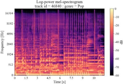
Fig. 1. Log-Mel spectrogram.
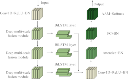
Fig. 2. Overall architecture of the Bi-HybridNet model.
3.2. Bi-HybridNet Model
3.2.1. Overall Architecture
Building on the ECAPA-TDNN framework, we propose the Bi-HybridNet model, which integrates a deep multi-scale fusion module with a BiLSTM layer. First, the deep multi-scale fusion module extracts richer feature representations and adjusts the relationships between channels using an adaptive mechanism to improve the classification accuracy of small datasets. To address the issue of temporal information loss, we developed Bi-HybridNet by incorporating a BiLSTM layer that captures critical sequential dependencies through both forward and backward passes. The overall architecture of Bi-HybridNet is shown in Fig. 2.
3.2.2. Deep Multi-Scale Fusion Module
Drawing inspiration from the inception architecture, we enhanced the original SE-Res2Block module to construct a deep multi-scale fusion module. The conventional SE-Res2Block module comprises multiple 1D convolutional layers, batch normalization (BN) layers, and squeeze-and-excitation (SE) modules. Although this structure combines ResNet’s residual connections with channel-wise attention mechanism of SE-NET and has demonstrated effectiveness in various classification tasks, its feature extraction capability remains limited for tasks with scarce training data.
To address this limitation, a novel multi-scale fusion module that replaces the original 1D convolution is proposed. Our module splits channel dimensions into multiple groups, with each group processed using convolutional kernels of different sizes. Specifically, we employed a combination of \(1\times 1\) and \(1\times 3\) convolutions across different channel groups to enhance the feature representation capacity while increasing the network depth. This parallel architecture enables the network to learn features at multiple scales and receptive fields, thereby better capturing detailed and global information from the input.
The outputs from all the channel groups were subsequently concatenated to form the final output representation. This design ensures the comprehensive utilization of multi-scale features while significantly improving the expressive power of the model. Our multi-scale fusion module demonstrated superior adaptability to audio input data, exhibiting stronger feature representation capability and higher classification accuracy. Furthermore, by increasing the module depth and complexity, we achieved improved performance across various tasks. The architecture of the multi-scale fusion module is shown in Fig. 3.
Subsequently, multiple multi-scale fusion modules were connected to form a deep multi-scale fusion module. Each new deep multi-scale fusion module consists of six multi-scale fusion modules, as illustrated in Fig. 4.
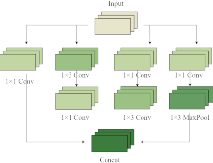
Fig. 3. Multi-scale fusion module.
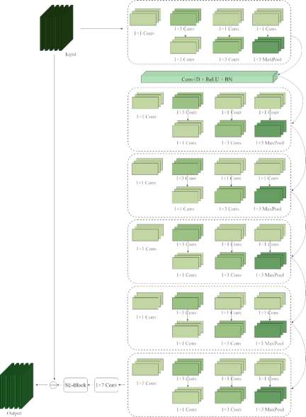
Fig. 4. Deep multi-scale fusion module.
3.2.3. BiLSTM Layer
The BiLSTM is a variant of long short-term memory (LSTM). The BiLSTM comprises two LSTMs operating in opposite directions. The forward LSTM layer processes the sequential data in the forward direction. At each time step, it receives the input and hidden states from the previous time step, updates the hidden states based on the gating mechanism, and generates an output. The backward LSTM layer operates similarly to the forward LSTM layer but processes the backward information flow of sequential data. It receives the input and hidden states from the subsequent time step and updates the hidden state while generating an output, following the same gating mechanism. The outputs of the forward and backward LSTM layers were then concatenated through a merging layer. This allows for the integration of forward and backward information to form a more comprehensive representation. Finally, the output layer performs specific tasks such as classification or regression according to the requirements of the application. Its structure is shown in Fig. 5.
In Fig. 5, \(x_{0}, x_{1}, x_{2}, \dots, x_{i}\) represent the inputs to the BiLSTM layer. Within the BiLSTM layer, the forward LSTM processes data starting from the beginning of the input sequence, whereas the backward LSTM processes data starting from the end of the input sequence.
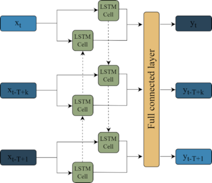
Fig. 5. Structure of the BiLSTM layer.
4. Experimental Results
4.1. Evaluation Metrics
To evaluate the performance of the proposed model, we employed accuracy, precision, recall, and F1-score. Specifically, for the multiclass music genre classification task, we adopted the macro-F1 metric to ensure a fair assessment across all genres. As defined in Eqs. (6) and (7), the precision and recall were calculated as the arithmetic means of the values for each class. Consequently, the F1-score was derived from the macro-averaged precision and recall, considering all eight genres equally, regardless of their sample distribution. The accuracy rate of the classifier refers to the proportion of correctly predicted samples to the total number of samples. The formula for calculating the accuracy rate is as follows:
Precision is the ratio of the number of samples correctly predicted as positive classes to the total number of samples predicted as positive classes. The formula for calculating the precision is as follows:
Recall is the ratio of the number of samples correctly predicted to be in the positive category to the number of samples in all true positive categories. It measures the degree of coverage of the model for samples in the positive category, that is, the model’s ability to recognize samples in the positive category. The formula for recall is as follows:
F1-score is the reconciled average of precision and recall, which is a comprehensive evaluation of the performance of the classification model, and is a weighted average of precision and recall, which considers the accuracy and coverage of the model simultaneously. The formula for calculating the F1-score is as follows:
The confusion matrix is shown in Table 1.
| Real positive results | Real negative results | |
| Predicting positive outcomes | \(\mathit{TP}\) | \(\mathit{FP}\) |
| Predicting negative outcomes | \(\mathit{FN}\) | \(\mathit{TN}\) |
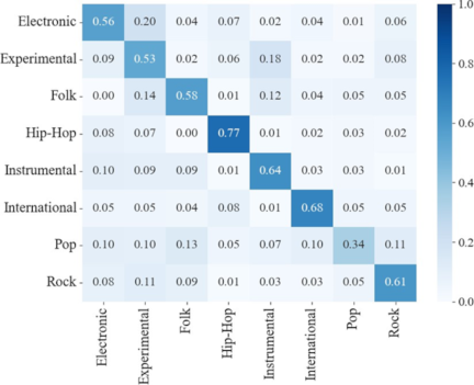
Fig. 6. Confusion matrix of the HybridNet model.
4.2. Experimental Results and Analysis
4.2.1. Training Process of the Bi-HybridNet Model
The variations in the accuracy and loss during the training process of the HybridNet model are shown in Fig. 6.
As illustrated in Fig. 6, the proposed HybridNet model demonstrates satisfactory overall accuracy in music genre classification, indicating its general effectiveness in capturing distinguishing features across different genres. However, upon closer examination of the performance in individual categories, it becomes evident that certain genres—specifically Pop, Experimental, Electronic, and Instrumental—are not classified as accurately as desired. The model experienced particular difficulty in distinguishing between these genres, which limited its overall classification precision. This limitation is largely attributable to the intrinsic characteristics of Pop music, which is often a genre of blended elements from various musical styles. Consequently, Pop shares a significant feature overlap with other genres such as Electronic and Instrumental, making it challenging for the model to clearly differentiate between them based solely on the extracted features.
To address this limitation, we introduced an enhanced Bi-HybridNet model, as shown in Fig. 7. This improved architecture incorporates a BiLSTM layer, which allows the model to effectively capture both forward and backward contextual dependencies within the input data. By integrating the temporal context in both directions, the BiLSTM layer enhances the model’s ability to form more comprehensive and nuanced feature representations. This leads to better discrimination between similar genres by modeling long-range patterns and subtle stylistic differences, which may have been missed by the original HybridNet. Consequently, Bi-HybridNet achieved noticeable improvements in the classification accuracy across all genres, particularly for those that were previously misclassified more frequently. Overall, this architectural enhancement significantly boosts the performance of the model, resulting in a more robust and reliable music genre classification system.
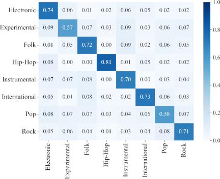
Fig. 7. Confusion matrix of the Bi-HybridNet model.
| ECAPATDNN | Deep multi-scale fusion module | BiLSTM | Accuracy | F1-score |
| \(✓\) | 82.65% | 0.563 | ||
| \(✓\) | \(✓\) | 84.16% | 0.579 | |
| \(✓\) | \(✓\) | 85.72% | 0.587 | |
| \(✓\) | \(✓\) | \(✓\) | 86.92% | 0.612 |
4.2.2. Ablation Studies
To verify the effectiveness of each component of the proposed Bi-HybridNet, ablation studies were conducted on an FMA-small dataset. Table 2 summarizes the performance of the baseline ECAPA-TDNN and the incremental improvements introduced by the deep multi-scale fusion module and BiLSTM layer.
As shown in Table 2, the baseline ECAPA-TDNN achieved an accuracy of 82.65% and an F1-score of 0.563.
Impact of multi-scale fusion: By incorporating a deep multi-scale fusion module, the model integrates features from the log-Mel spectrogram at varying scales. This module employs parallel \(1\times 1\) and \(1\times 3\) convolutions to enrich the feature expressiveness and expand the receptive field. This allows the network to capture fine-grained details and global structural information simultaneously. Consequently, the model achieved a 1.51% increase in accuracy and a 0.016 improvement in the F1-score compared to the baseline.
Impact of BiLSTM: The introduction of the BiLSTM layer allows the model to capture bidirectional temporal dependencies within an audio sequence. By aggregating forward and backward contextual information, BiLSTM forms a more comprehensive representation of the spectral evolution. This resulted in a significant gain, boosting the accuracy by 3.07% and F1-score by 0.024 over the baseline.
Combined Effect: When modules are integrated (Bi-HybridNet), the model effectively merges the multi-scale spatial features with bidirectional temporal dynamics. This synergistic combination yielded the best performance, with a total improvement of 4.27% in accuracy and 0.049 in F1-score to the standalone ECAPA-TDNN.
Discussion on Metrics: The reported F1-score (approx. 0.61) differs from higher values (0.75–0.82) often reported in studies utilizing simpler datasets like GTZAN. This discrepancy is primarily attributed to the complexity of the FMA-small dataset, which comprises 8000 tracks with diverse audio characteristics and professional curation, presenting a significantly more challenging classification task than smaller benchmarks. Therefore, the absolute metrics reflect the robustness of the model on a complex real-world benchmark.
The reported F1 score (approximately 0.6) differs from the higher values (0.75–0.82) often reported in previous BiLSTM-based studies. This discrepancy is primarily attributed to differences in dataset complexity and experimental protocols. Unlike simpler datasets (e.g., GTZAN) used in previous studies, we utilized the FMA-small dataset, which contains a larger scale of 8000 tracks with more complex audio characteristics and professional curation. Furthermore, our preprocessing involves extracting the log-Mel spectrum to capture fine-grained time-frequency features, which presents a more challenging task for classification compared to simpler feature inputs. Therefore, although the absolute F1 value may appear low, it reflects the performance of the model on a more robust and challenging benchmark.
4.2.3. Comparative Experiments
To validate the effectiveness of the proposed architecture, we compared Bi-HybridNet with various classical baseline methods, including standard recurrent networks (LSTM, GRU, and Bi-GRU), convolutional networks (ResNet), and Transformer-based architectures. In addition, we evaluated hybrid configurations (e.g., ResNet combined with LSTM/GRU) to assess the benefits of fusing spectral and temporal features.
The experimental results in Table 3 demonstrate that Bi-HybridNet performed well among the tested architectures. While the standard Transformer model captures global dependencies, it underperforms compared with our method, likely owing to the lack of an inductive bias suitable for local spectral feature extraction in audio. Similarly, while hybrid models such as ResNet + Bi-GRU show competitive results, they fall short of the performance achieved by our specialized SE-Res2Block and multi-scale fusion design.
| Model | Accuracy | F1-score |
| LSTM | 67.22% | 0.447 |
| GRU | 70.25% | 0.495 |
| Bi-GRU | 71.69% | 0.503 |
| ResNet | 77.14% | 0.556 |
| Transformer | 72.52% | 0.518 |
| ResNet + LSTM | 79.25% | 0.547 |
| ResNet + GRU | 81.03% | 0.562 |
| ResNet + Bi-GRU | 83.26% | 0.575 |
| Bi-HybridNet | 86.92% | 0.612 |
It should be noted that as performance on standard benchmark datasets for music genre classification may already be close to saturation, this study focuses more on providing a practical technical solution than on pursuing absolute state-of-the-art performance. The better performance of Bi-HybridNet can be attributed to two core designs: (1) deep multi-scale feature extraction: Unlike standard CNNs, the fusion module in the proposed method captures spectral patterns at multiple resolutions and is enhanced by an attention mechanism that suppresses irrelevant background noise; (2) bidirectional contextual modeling in which the BiLSTM layer provides a complete understanding of the sequential structure, integrating past and future contexts to resolve ambiguities in genre boundaries. These results confirmed that Bi-HybridNet achieved an optimal balance between precision and recall, particularly in complex and imbalanced music genres.
5. Conclusion
With the development of Internet platforms and smart devices, the digital music market has experienced rapid growth in terms of both music distribution and the user base. The effective genre classification of massive music collections facilitates personalized recommendations on music platforms, enhances user satisfaction with song recommendations, and promotes the development of the music industry. To improve the accuracy of music genre classification, this paper proposes a Bi-HybridNet model with the following main contributions:
-
(1)
Deep multi-scale fusion module: To extract comprehensive and discriminative audio features for improved music-genre classification, we proposed a deep multi-scale fusion module. This module employs convolutional kernels of varying sizes for feature extraction, where different channels utilize combinations of \(1\times 1\) and \(1\times 3\) convolutions to enhance the feature representation and deepen the model. This parallel architecture enabled the network to learn features at multiple scales and in receptive fields, effectively capturing both fine-grained details and global information in the log-Mel spectrum. In addition, this structure ensures robust performance, even for small datasets.
-
(2)
BiLSTM layer for long-term dependency modeling: To strengthen the ability of the model to capture long-term dependencies, we incorporated a BiLSTM layer. As a variant of recurrent neural networks, BiLSTM effectively models temporal relationships in sequential data. By integrating BiLSTM into the residual structure of the HybridNet model, we leveraged its capability to process sequential information bidirectionally.
It should be emphasized that this study is positioned as solid technical application research, providing a practical solution for music genre classification tasks. Although the performance improvement on standard benchmark datasets is limited, it offers a certain reference value for feature extraction strategies and temporal modeling methods, providing beneficial insights for related research.
6. Limitations and Future Work
Despite the promising results achieved on the FMA-small dataset, this study had certain limitations. First, the generalization capability of the proposed model was evaluated using a single dataset. Although the FMA-small is a challenging and widely recognized benchmark, its performance on other datasets (e.g., GTZAN and MagnaTagATune) remains to be verified. Consequently, there is a potential risk that the model may adapt specifically to the characteristics of FMA-small dataset.
Second, regarding computational efficiency, although our model focuses on improving the accuracy through multi-scale fusion and BiLSTM, we acknowledge that this may come at the cost of higher computational complexity. Although we did not quantify the exact inference speed or memory footprint in this study, we recognize that it is crucial for real-time or edge-device applications. Therefore, future work will include a detailed analysis of the computational cost (e.g., FLOPs and inference latency) and the exploration of model compression techniques to enhance practical utility.
Acknowledgments
This study was supported by Key Scientific Research Project of Suzhou University (No.2025yzd27), Anhui Provincial Department of Education Communication Engineering Teaching Team Project (No.2021jxtd291), and Quality Engineering Project of Suzhou University (No.szxy2024xwjy02).
- [1] International Federation of the Phonographic Industry, “Global music report 2023,” 2023. https://globalmusicreport.ifpi.org/ [Accessed February 26, 2024]
- [2] C. Cortes and V. Vapnik, “Support-vector networks,” Mach. Learn., Vol.20, No.3, pp. 273-297, 1995. https://doi.org/10.1007/BF00994018
- [3] B. Matityaho and M. Furst, “Neural network based model for classification of music type,” 18th Conv. Electr. Electron. Eng. Isr., Session No.4.3.4, 1995. https://doi.org/10.1109/EEIS.1995.514161
- [4] D.-N. Jiang, L. Lu, H.-J. Zhang, J.-H. Tao, and L.-H. Cai, “Music type classification by spectral contrast feature,” Proc. IEEE Int. Conf. Multimed. Expo, Vol.1, pp. 113-116, 2002. https://doi.org/10.1109/ICME.2002.1035731
- [5] C. Laurier and P. Herrera, “Audio music mood classification using support vector machine,” MIREX Task Audio Mood Classif., pp. 2-4, 2007.
- [6] Y. Panagakis, C. Kotropoulos, and G. R. Arce, “Non-negative multilinear principal component analysis of auditory temporal modulations for music genre classification,” IEEE Trans. Audio Speech Lang. Process., Vol.18, No.3, pp. 576-588, 2010. https://doi.org/10.1109/TASL.2009.2036813
- [7] Y. M. G. Costa, L. S. Oliveira, A. L. Koerich, F. Gouyon, and J. G. Martins, “Music genre classification using LBP textural features,” Signal Process., Vol.92, No.11, pp. 2723-2737, 2012. https://doi.org/10.1016/j.sigpro.2012.04.023
- [8] S. Sugianto and S. Suyanto, “Voting-based music genre classification using melspectogram and convolutional neural network,” 2019 Int. Semin. Res. Inf. Technol. Intell. Syst. (ISRITI), pp. 330-333, 2019. https://doi.org/10.1109/ISRITI48646.2019.9034644
- [9] Y. Atahan et al., “Music genre classification using acoustic features and autoencoders,” 2021 Innov. Intell. Syst. Appl. Conf. (ASYU), 2021. https://doi.org/10.1109/ASYU52992.2021.9598979
- [10] X. Liu, S. Song, M. Zhang, and Y. Huang, “MATT. A multiple-instance attention mechanism for long-tail music genre classification,” 2022 IEEE Int. Conf. Syst. Man Cybern. (SMC), pp. 782-787, 2022. https://doi.org/10.1109/SMC53654.2022.9945477
- [11] B. Liang and M. Gu, “Music genre classification using transfer learning,” 2020 IEEE Conf. Multimed. Inf. Process. Retr. (MIPR), pp. 392-393, 2020. https://doi.org/10.1109/MIPR49039.2020.00085
- [12] L. G. Hafemann, L. S. Oliveira, and P. Cavalin, “Forest species recognition using deep convolutional neural networks,” 22nd Int. Conf. Pattern Recognit., pp. 1103-1107, 2014. https://doi.org/10.1109/ICPR.2014.199
- [13] W. Zhang, W. Lei, X. Xu, and X. Xing, “Improved music genre classification with convolutional neural networks,” Proc. Interspeech 2016, pp. 3304-3308, 2016. https://doi.org/10.21437/Interspeech.2016-1236
- [14] C. Senac, T. Pellegrini, F. Mouret, and J. Pinquier, “Music feature maps with convolutional neural networks for music genre classification,” Proc. 15th Int. Workshop Content-Based Multimed. Index. (CBMI), Article No.19, 2017. https://doi.org/10.1145/3095713.3095733
- [15] K. Choi, G. Fazekas, M. Sandler, and K. Cho, “Transfer learning for music classification and regression tasks,” arXiv:1703.09179, 2017. https://doi.org/10.48550/arXiv.1703.09179
- [16] H. Yang and W.-Q. Zhang, “Music genre classification using duplicated convolutional layers in neural networks,” Proc. Interspeech 2019, pp. 3382-3386, 2019. https://doi.org/10.21437/Interspeech.2019-1298
- [17] C. Liu, L. Feng, G. Liu, H. Wang, and S. Liu, “Bottom-up broadcast neural network for music genre classification,” Multimed. Tools Appl., Vol.80, No.5, pp. 7313-7331, 2021. https://doi.org/10.1007/s11042-020-09643-6
- [18] G. Song, Z. Wang, F. Han, S. Ding, and M. A. Iqbal, “Music auto-tagging using deep Recurrent Neural Networks,” Neurocomputing, Vol.292, pp. 104-110, 2018. https://doi.org/10.1016/j.neucom.2018.02.076
- [19] Z. Wang, S. Muknahallipatna, M. Fan, A. Okray, and C. Lan, “Music classification using an improved CRNN with multi-directional spatial dependencies in both time and frequency dimensions,” 2019 Int. Jt. Conf. Neural Netw. (IJCNN), 2019. https://doi.org/10.1109/IJCNN.2019.8852128
- [20] R. Yang, L. Feng, H. Wang, J. Yao, and S. Luo, “Parallel recurrent convolutional neural networks-based music genre classification method for mobile devices,” IEEE Access, Vol.8, pp. 19629-19637, 2020. https://doi.org/10.1109/ACCESS.2020.2968170
This article is published under a Creative Commons Attribution-NoDerivatives 4.0 Internationa License.