
Research Paper:
Size Classification for Software Maintenance Projects Through a Simplified Minimalist Machine Learning Algorithm
Cuauhtémoc López-Martín*
 , Cornelio Yáñez-Márquez**,†
, and Ali Bou Nassif***
, Cornelio Yáñez-Márquez**,†
, and Ali Bou Nassif***
*Department of Information Systems, Universidad de Guadalajara
Periférico Norte No.799 Núcleo Universitario, C. Prol. Belenes, Zapopan, Jalisco 45100, México
**Centro de Investigación en Computación, Instituto Politécnico Nacional
Av. Juan de Dios Bátiz S/N, Nueva Industrial Vallejo, Gustavo A. Madero, Ciudad de México 07738, México
†Corresponding author
***Department of Computer Engineering, University of Sharjah
P.O. Box 27272, United Arab Emirates

In the software engineering field, the size of projects is used as explanatory variable for predicting the effort, duration, defects, costs, or risks of a project. Thus, the software project size has been considered the most influential factor. A systematic mapping study on the use of categorical data in software prediction concludes that the use of categorical data as explanatory variable in prediction models is an important issue because in the first phases of the software development process, the information is expressed in a categorical manner rather than numerical; however, at date, software size has mostly been used in its quantitative form rather than in its categorical representation. Because the software enhancement maintenance has the highest impact on business, our purpose is to classify software enhancement projects from their size by applying a new model termed simplified minimalist machine learning (S-MML) algorithm, which belongs to the minimalist machine learning (MML) paradigm. S-MML reduces five attributes commonly used for sizing a software project to only one. The performance of the S-MML is compared to those obtained from three classifiers. Seven public datasets of projects obtained from an international public repository of software projects were used to train and test the classifiers. Results showed that the S-MML had a better f-measure than the other three classifiers for all of the datasets at 95% confidence. We can conclude that the S-MML can be applied to classify the size of software enhancement projects.
1. Introduction
One of the main challenges of the intelligence computing corresponds to a recent demand launched from several research international groups to the scientific community. This challenge consists in giving to the intelligent algorithms an explainable property 1,2. At date, it is explicitly accepted in the existence of very effective models for specific applications 3; however, at the same time, these models have been questioned due to their limited interpretability, as they are often regarded as “black boxes” 4.
The creativity in researchers has emerged by proposing several solutions to the mentioned challenge. The ideas have been reproduced in a lot of groups of researchers to answer this challenge 5, whose relevance has even been taken into account for the USA Defense Advanced Research Projects Agency, which creates pattern classification algorithms such that their decisions can be understandable (and believable) for final users 6.
Research groups have also been working in developing understandable machine learning (ML) models by publishing studios proposing the idea of a new paradigm termed minimalist machine learning (MML), whose purpose is to design simple and transparent models for the pattern intelligent classification task, such that these models can explain in a diaphanous manner what is happening with the classes of the patterns involved in the problem to be solved 7,8.
The premises under the minimalist paradigm aim against those ones assumed in the middle of 1990s, whose epoch relevant models were proposed such as support vector machine (SVM) having the following premise: if the problem classes are non-linearly separable in a space of \(n\) dimensions, then a function kernel has to be identified for transforming the data to a space having more dimensions, such that there exists the possibility of that in this complex space, the problem data are separable 9.
It is relevant to stand out that MML paradigm has as objective to tackle the challenge of achieving understandable intelligent algorithms. This achievement is performed through the simplification of data representation spaces; that is, achieving the reduction of the space dimensions.
In the present study, we introduce a MML model termed simplified minimalist machine learning (hereafter S-MML), which takes advantage of the data representation for generating a simple, effective, and explainable classifier.
Regarding S-MML application, the process phases of a software project are definition (software requirements, and software planning), development (design, coding, and testing), and maintenance. There are several types of software maintenance, such as enhancement, consultive, training, evaluative, reformative, updative, groomative, preventive, performance, adaptive, reductive, and corrective. Among them, the enhancement type has the highest impact on business over the others types 10. It is performed when new functionality is added or existing functionality is changed or deleted 11. In the present study, we used data of software enhancement projects selected from an international public repository of software projects (i.e., ISBSG, whose preprocessing is described in Section 4).
The project software requirements phase is related to the elicitation, analysis, specification, and validation of software requirements, as well as to the management of them 12. Once software requirements are specified, the software project size is then calculated and used to predict the effort (i.e., person-months) 13, duration (mainly measured in months) 14, defects 15, or monetary costs of software projects 16,17. The size can be obtained from either lines of code (LOC) or functional size measurement (FSM) 18. The latter has been defined as the “size of the software derived by quantifying the functional user requirements” 19, and as “a technique for evaluating the size of a body of functional requirements” 20. FSM has been preferred over LOC because it is difficult to predict the LOC in advance of development phase 20. There have been proposed several standards for FSM such as IPPUG, NESMA, FiSMA, and COSMIC 21. Actually, the functional sizing has been reported as the technique most documented 22.
Project size is very important due to the following two aspects:
-
1)
It can explain between the 80% and 90% of the development effort of a project, while all the other factors together between 10% and 20% 20.
-
2)
It has been considered the most influential factor when software is predicted 23.
Categorical values, also termed qualitative values 24 or linguistic values 25 generalize numbers, and are easier to understand than numerical values 26. In accordance with the scale types (i.e., nominal, ordinal, interval, and ration), categorical values correspond to nominal or ordinal type 27. The latter ranks the categories in a certain order as follows for a software project size:
-
1)
LOC has been classified in small, intermediate, medium, large, and very large 23.
-
2)
FSM has been classified in extra-extra-small, extra-small, small, medium, large, extra-large, extra-extra-large, and extra-extra-extra-large 21.
The classification of software project size in categories has widely been recommended 20,23. Categorical data have been studied in the statistics field since more than eight decades ago 28,29,30, whereas the software engineering field is more recent; a systematic mapping study on the use of categorical data in software development effort prediction involves 27 studies published between 1997 and 2019. It concludes that the use of categorical data as explanatory variables in prediction models is an important issue because in the first phases of the software development process, the information is expressed in a categorical manner rather than numerical. The authors of the mentioned systematic review did not identify any case study regarding the use of categorical values in prediction models, therefore, they suggest to the researchers and practitioners to cooperate for exploring this issue 31. Accordingly, our study contributes to the mentioned suggestion, in the sense of proposing the S-MML for classifying the size of a software enhancement project into a category.
In accordance with statistics, it is recommended using more than an attribute for describing a factor 32, thus, the S-MML is based on five FSM attributes.
In our study, the size by software project was selected from the ISBSG dataset Release 2018 21. The ISBSG reports the classification by project from its size measured in function points. There exists unadjusted function points (UFP), and adjusted function points (AFP). UFP are calculated from the following five variables: external inputs (EI), external outputs (EO), external inquiries (EQ), internal logical files (ILF), and external interface files (EIF). These five variables are calculated by using complexity tables and diagrams which represent the software functional requirements 33. Once UFP value is obtained, an adjust factor is calculated from other fourteen variables related to software non-functional requirements, then this adjust factor is used for adjusting that UFP value, and then the AFP value is obtained. The ISBSG dataset reports individually the mentioned five variables, and an adjust factor value obtained from the fourteen variables is reported. In the present study, the five mentioned variables are used for classifying the projects.
In our study, the project size was selected from the ISBSG dataset Release 2018 21, which classifies software projects according to FSM expressed in function points 19,20. The UFP are computed from five functional components: EI, EO, external inquiries (EQ), ILF, and EIF 21,33. These components quantify the functional user requirements of the system by counting data movements and logical data groups under standardized complexity criteria 19,33.
Each of the five variables (EI, EO, EQ, ILF, EIF) represents a quantitative indicator of functional scope and jointly determines the UFP value prior to adjustment by non-functional factors 21. Following statistical recommendations to describe a factor using multiple attributes 32, these FSM components are treated as explanatory variables in the size classification task. Within the S-MML framework, the five-dimensional representation is transformed through arithmetic summation into a single real-valued scalar, preserving the overall functional magnitude while reducing the dimensionality of the representation space. This scalar is then used to classify projects into the ISBSG categorical size levels defined by standardized function point intervals 21.
In general, S-MML proposes the representation space simplification through simple transformations (such as arithmetic operations) until achieving the plane. In our study, the patterns (i.e., software projects) originally consist of five components (EI, EO, EQ, ILF, and EIF) that, with a new representation of these five attributes, they are simplified by a simple real number. This is achieved through a simple (but extremely important in mathematics) arithmetic operation: the sum of real numbers.
In our study, the performance of the S-MML is compared to those obtained from discriminant analysis (DA), SVM, and multilayer perceptron (MLP) classifiers based on the following reasons:
- 1)
- 2)
- 3)
In the present study, the performance measure used for S-MML, DA, SVM, and MLP is \(f\)-measure, which is calculated from precision, and sensitivity measures.
The hypotheses to be tested in our study are the following:
-
\(H_0\):
The size classification prediction accuracy with S-MML is statistically equal than the accuracy obtained with DA, SVM, and MLP.
-
\(H_1\):
The size classification prediction accuracy with S-MML is statistically not equal than the accuracy obtained with DA, SVM, and MLP.
The rest of this study is organized as follows: Section 2 describes the studies related to software size. Section 3 details the S-MML. Since the three classifiers applied in our study are well-known for the computer science community, they are briefly described in Section 4. This section also includes the criteria for selecting the data sets of software projects, as well as the definition of the performance measures for classifiers. Section 5 shows the results obtained when S-MML is applied and resting of the classifiers. Finally, Section 6 presents the discussion including our conclusions, limitations, and validity threats of our study, as well as the proposed future work.
2. Related Works
The research on the software project size has been approached from a several points of view, such as methods to estimate it, the effect on quality, the factors that affect its estimation, the applications of models for estimate it, its relationship with the productivity, its relationship with the accuracy when applied to effort or defect prediction, its relationship with the software contract selection, as well as the equivalence between types of software size. As for size classification, we identified some references classifying it from two types of measures: FSM and LOC. These studies are briefly described next.
Catal and Diri 40 analyze the effect of dataset size, metrics set, and feature selection techniques in the context of software fault prediction. They apply ML learning classifiers concluding that random forests was the better classifier when large datasets were used, and naive Bayes when small datasets were used, whereas the artificial immune recognition system was the best one when the method-level metrics were used.
El Emam et al. 41, demonstrate that the size of object-oriented classes affects the software quality (i.e., defects). They conclude that there exists a continuous relationship between class size and faults.
Fink and Lichtenstein 42 analyze the importance of the software project size on the software contract selection. They develop two models: the first model is based on that the effect of project size on contract choice is mediated by project detail, whereas in the second one, the effect of project size on contract choice is moderated by project detail and vendor familiarity. They use data from a bank, and their results confirm that both mediation and moderation are accepted.
Kitchenham and Mendes 43 use the software size measures to analyze the software productivity. They propose size/effort as productivity measure for web applications. They conclude that the mentioned measure is the most appropriate when regression model is used for effort prediction.
Tan et al. 44, propose a size estimation method based on multiple linear regression model using to LOC. They used software projects from industry and open-source systems.
Lind and Heldal 45 apply the COSMIC FSM method for sizing embedded software components of the automotive industry. They perform a correlation analysis between FSM and software code size finding a strong correlation between them.
MacDonell 46 applies fuzzy logic for software source code sizing. He applies clustering and rule extraction methods to generate the fuzzy models from a set of projects and then he compares the accuracy of them to those obtained from statistical regression models. He concludes that fuzzy predictive models outperform statistical regression models.
Ochodek 47 proposes the approximation between two types of FSM size (i.e., COSMIC and IFPUG FPA) from UML use-case diagrams or a list of use-case names. He concludes that use case diagrams could be used to obtain an early approximation of the application size.
Pendharkar 48 identifies factors that may affect the size of an object-oriented software component, and then he determines the effect of these factors on the prediction of the size of the software component. He uses regression trees used to learn decision rules.
Verner and Tate 49 propose a bottom-up approach to software size estimation. They identify factors associated to software size. Then they use equations for selecting explanatory variables used for size estimation. The bottom-up approach firstly consists in sizing individual software components, and then they integrate subsystems and system sizes.
In accordance with references related to software size classification, we identify the following three references.
Aguilar et al. 50 classify the size of software projects based on LOC as shown in Table 1.
| Classification | Size (LOC) |
| Micro | 1600–9,600 |
| Small | 9,601–38,400 |
| Medium | 38,401–960,000 |
| Large | 960,000 or more |
Alyahya et al. 23 classify the size in accordance with their thousands of LOC (KLOC) as shown in Table 2.
| Classification | Size (KLOC) |
| Small | 2 |
| Intermediate | 8 |
| Medium | 32 |
| Large | 128 |
| Very large | 512 |
The ISBSG classifies the size based on FSM (i.e., AFP) as shown in Table 3 21.
| Classification | Size (AFP) |
| Extra-extra-small | 0 and \(<10\) |
| Extra-small | 10 and \(<30\) |
| Small | 30 and \(<100\) |
| Medium1 | 100 and \(<300\) |
| Medium2 | 300 and \(<1000\) |
| Large | 1,000 and \(<3,000\) |
| Extra-large | 3,000 and \(<9,000\) |
| Extra-extra-large | 9,000 and \(<18,000\) |
| Extra-extra-extra-large | 18,000 or more |
3. S-MML Model
The year of 2020 marks the birth MML paradigm. The fundamental premises and the basic concepts as well as the ideas that support the MML were recently published 7. The MML paradigm starts from the following fundamental premise: “it is possible to solve the Euclidean plane any classification problem without matter the dimension of its patterns.” This MML premise could sound improbable for anybody who knows the different approaches and algorithms of the state-of-the-art pattern classification. However, we without a doubt have verified the effectiveness of MML models and algorithms before the year of 2020. It is necessary to emphasize that, without exception, all of mentioned models and algorithms have been grounded on that adventurous and disruptive MML premise.
In order to contextualize the presentation of our new S-MML model, we explain and illustrate the answer given to following genuine and valid question 7: how the MML models and algorithms do achieve to solve classification problems in one Cartesian plane regardless of the size of the patterns? Is it possible to achieve it from a dataset whose patterns have, as example, a dimension higher than 1,000? The answer is: yes.
Firstly, let \(D\) a dataset, which is designed for the classification task in ML. Let us also assume that \(D\) contains a total of \(n\) patterns distributed in two classes, and that each pattern is made up for \(n\) numeric attributes; that is, the dimension of the patterns is \(n\).
The common practice in solving problems in the area of supervised pattern classification is to apply a validation method to the dataset. The result of applying the validation method is a partition of the dataset \(D\) into two disjoint subsets: a training or learning set \(L\) and a test set \(T\) that change by algorithm iteration. The number of iterations that the algorithm performs is directly determined by the choice of the validation method to be applied. Although in the state of the art there exists several validation methods, one of the most useful when used in small datasets is the leave-one-out cross-validation (LOOCV).
We exemplify with the following algorithm 7: let a pattern \(P\) (having an \(n\) dimension) in the subset \(L\). Then, the following two very simple operations are applied to that \(P\) training pattern: standard deviation, and mean. Afterwards, the standard deviation value (std(\(P\))) is located on the \(x\)-axis, whereas the mean value (mean(\(P\))) is located on the \(y\)-axis. As result, the ordered pair (std(\(P\)), mean(\(P\))) is plotted in the Cartesian plane, regardless of the size of \(n\)!
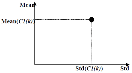
Fig. 1. Graphical representation of the \(k\)-th learning pattern for the class 1 (where C1 corresponds to class 1 from \(D\)).
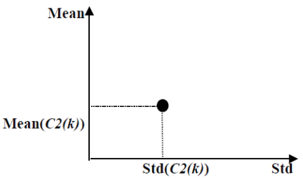
Fig. 2. Graphical representation of the \(k\)-th learning pattern for the class 2 (where C2 corresponds to class 2 from \(D\)).
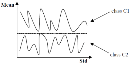
Fig. 3. Ideal performance for MML paradigm (the dotted horizontal line separates the classes).
Figure 1 depicts the \(k\)-th learning pattern for the class 1, whereas Fig. 2 shows the \(k\)-th learning pattern for the class 2.
The ideal issue regarding MML paradigm model is to achieve the separation between the two classes on the Cartesian plane as shown in Fig. 3.
How the dotted horizontal line that separates the classes in Fig. 3 is obtained? The answer is: using a basic (minimalist) operation by calculating the minimum of the superior class (i.e., class 1 in Fig. 3) and the maximum of the inferior class (i.e., class 2 in Fig. 3) then the arithmetic mean from them is calculated, which corresponds to the height of the dividing line. We can observe an interesting issue in the ideal case shown in Fig. 3: the minimum value of the superior class is above maximum value of the inferior class. When a test pattern is being located, we can observe which side this pattern belongs to: if it is located above, a class 1 is assigned to the pattern, otherwise, a class 2 is assigned. Since the procedure is supervised, the practitioner can determine if there is or not an error. Actually, using this result, the classifier performance is calculated.
Unfortunately, this result is not common in real classification problems but not separated between classes when the steps regarding the described algorithm are performed. Thus, the minimum value of the superior class is under the maximum value of the inferior class, which means that there is an overlap of classes. This situation causes a low performance in the classifier as the overlap is greater.
The original MML model has slightly been modified showing a competitive result with other state-of-the-art classifiers by classifying images of brain hemorrhages 51. Actually, the original MML model outperforms the more important classifiers.
In the present study, the new S-MML model we introduce has been inspired by the original MML model 7. The “S” in the acronym means “simplified,” that is, the S-MML is a simplified model with respect to the original MML model. This simplification involves the following two manners that exacerbate the “minimalist” character into the MML paradigm models:
-
1)
We have discovered that we can omit the use of the standard deviation, and only use a simple operation. However, if we remain only simple operation: how to achieve the representation in the Cartesian plane? Substituting the value of the standard deviation in the \(x\)-axis by intervals consistently spaced. The number of these intervals coincides with the number of patterns found in the plotted class. A remarkable fact is that the elimination of one of the two operations of the original model does not affect the efficacy of the new model even though its efficacy increases.
-
2)
We have discovered that we can use a simpler operation than the mean, which one? We do not use the mean anymore, but the sum.
Without generality loss, we assumed that the dataset consists of two classes mutually exclusive.
3.1. S-MML Learning Phase
-
1)
All components by pattern (i.e., by software enhancement project) are added. This step achieves a new representation of that pattern by means of a real number.
-
2)
The values by class are graphed on the plane, taking into account intervals consistently spaced on \(x\)-axis.
-
3)
A threshold \(u\) is calculated as follows: the minimum value from the class 2 is added to the maximum value of the class 1. The result of this addition is divided by two.
Figures 4 and 5 are based on a dataset used in the present study (described in Table 4). They correspond to the training phase while the LOOCV is performed, and involve 38 software enhancement projects developed in MidRange and coded in third programming generation languages. In Figs. 4 and 5, the patterns number 22 and number 6 of the class M1 (blue) are excluded as test pattern, respectively.
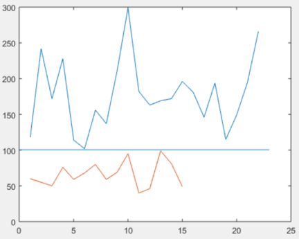
Fig. 4. The pattern number 22 of the class M1 (blue) is excluded as test pattern.
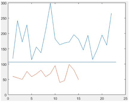
Fig. 5. The pattern number 6 of the class M1 (blue) is excluded as test pattern.
| DP | LT | NP | SVM | MLP | |||
| KT | PV | NHL | LR | M | |||
| MF | 3GL | 204 | Polynomial | \(\gamma=0.2\), \(c_0=0.8\), \(d=2\), \(C=1\) | 1 | 0.03 | 0.2 |
| Multi | 3GL | 61 | Polynomial | \(\gamma=0.3\), \(c_0=0.4\), \(d=2\), \(C=1.2\) | 2 | 0.05 | 0.4 |
| Multi | 4GL | 38 | Polynomial | \(\gamma=0.8\), \(c_0=0.8\), \(d=2\), \(C=1.5\) | 2 | 0.7 | 0.8 |
| MF | 3GL | 50 | Linear | \(C=1.1\) | 1 | 0.7 | 0.1 |
| MR | 3GL | 139 | Polynomial | \(\gamma=1.2\), \(c_0=1.5\), \(d=3\), \(C=1.3\) | 1 | 0.02 | 0.5 |
| Multi | 3GL | 47 | Polynomial | \(\gamma=0.45\), \(c_0=0.5\), \(d=2\), \(C=0.9\) | 2 | 0.9 | 0.1 |
| PC | 4GL | 29 | Linear | \(C=1\) | 1 | 0.8 | 0.7 |
3.2. S-MML Classification Phase
The data representation previously described allows an S-MML classification phase to be extremely simple (minimalist):
-
1)
Let a test pattern \(p\), whose components are added such that \(p\) is represented by a real number \(r\).
-
2)
The \(r\) value is compared to threshold \(u\). If \(r>u\), then \(p=\) class 2, if \(r<u\) then \(p=\) class 1.
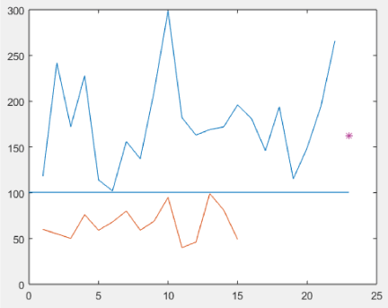
Fig. 6. A correct classification for the S-MML.
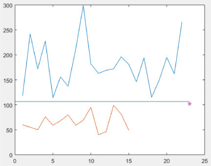
Fig. 7. An incorrect classification for the S-MML.
Figures 6 and 7 are based on the same dataset used in the Figs. 4 and 5. In Fig. 6 the pattern number 22 of the class M1 (blue) is excluded as test pattern. We can observe that when the test pattern is located, it (pink asterisk) is above the straight decision. Thus, this test pattern is assigned to the class M1 (blue), that is, to which it really belongs. We can then conclude that it corresponds to a correct classification for the S-MML. As for Fig. 7, the pattern number 6 of the class M1 (blue) is excluded as test pattern. In this case, we can observe that when the test pattern is located, it (pink asterisk) is under the straight decision, and this test pattern is assigned to the incorrect (red) class. Since the test pattern really does belong to the class M1 (blue), it is considered as an error for the S-MML.
4. Materials and Methods
In this section, we present the materials and methods that demonstrate the strengths of our original proposal (S-MML) by comparing the results with state-of-the-art algorithms when applied to datasets related to software maintenance projects. This includes state-of-the-art algorithms, datasets, and performance metrics.
4.1. Classifiers
We have included brief descriptions of three of the most relevant state-of-the-art classification algorithms.
4.1.1. DA
DA is a traditional statistical method for classification. In addition to the multivariate data, it assumes prior knowledge of class memberships. This dataset of classes is used for a training phase, whereas only the multivariate information without class membership information is used for a test dataset. The objective of the DA is to predict the class memberships for the test dataset software projects through a Fisher discriminant rule obtained from the training dataset. The DA method is described as follows 35.
Suppose that \(n\) software projects correspond to the training dataset; and that these are compositions with \(D\) compositional parts.
The \(n\) software projects originate \(g \ge 2\) different groups, and the sample sizes of the groups are \(n_1,n_2,\dots,n_g\), with \(n_1+n_2+\dots+n_g=n\).
Let the notation \(x_{ij}\) to distinguish the software projects from the different groups, which corresponds to the column vector of the compositional information of the \(i\)-th software project (where \(i=1,\dots,n_j\), for the \(j\)-th group, with \(j=1,\dots,g\)).
Assume that (a) the \(g\) groups originate from \(g\) underlying populations \(\pi_1,\dots,\pi_g\), and (b) the \(j\)-th population has a certain prior probability \(p_j\), with \(p_1+p_2+\dots+p_g=1\). Therefore, \(p_j\) would correspond to the probability that a software project comes from population \(\pi_j\). In case of that training dataset reflects the structure of the populations, it is expected that \(n_j/n\) is close to \(p_j\) for all groups.
Because of DA is based on Euclidean geometry, isometric log-ratio coordinates are used to express the composed underlying data.
Thus, the vector with length \(D\) for the \(i\)-th software project from the \(j\)-th group, \(x_{ij}=(x_{i1}^{[j]},x_{i2}^{[j]},\dots,x_{iD}^{[j]})'\), is expressed in pivot coordinates as the following equation:
This equation results in the column vector to
DA has as an additional assumption that the \(j\)-th population \(\pi_{\textit{th}}\) can be represented by an density function \(f_j\), for \(j=1,2,\dots,g\), assumed to be a multivariate normal density with expectation \(\mu_j\) and covariance \(\Sigma_j\), where \(\mu_j\) is a vector of length \(D-1\), and \(\Sigma_j\) is a matrix of dimension \((D-1)\times (D-1)\), whose quantities are calculated from the training dataset. The objective of the DA is to predict the class memberships for the test dataset through a Fisher discriminant rule obtained from the training dataset.
It is important to note that DA is considered a classical statistical baseline in software engineering prediction studies. Different comparative studies have pointed out that any new intelligent model should at least outperform a traditional statistical approach to demonstrate practical relevance. In this sense, DA represents a well-established parametric classifier, grounded in statistical decision theory, and widely used in effort estimation and defect prediction contexts. Therefore, its inclusion allows to position S-MML with respect to a rigorous and historically accepted statistical reference.
4.1.2. SVM
Vapnik proposed the first SVM in 1963 52. Then, Boser et al. is modified in 1992 the original algorithm for non-linear classifiers from the kernel method 53. Afterwards, the most recent improvement on SVM was presented in 1995 by Vapnik 52.
The first SVM objective of SVM was firstly to deal with binary classification problems 53, and further SVM improvements allowed multi-class classification 52.
A SVM searches for the linear decision surface that separates two classes of input patterns (i.e., vectors). Then, a maximized margin between the linear decision surface (i.e., hyperplane) and the vectors (i.e., the support vectors) is performed. The optimal hyperplane improves the SVM classification by minimizing the error. That is, a SVM looks for a hyperplane that maximizes the margin of separation between classes with a minimum error. Since a kernel function represents the patterns in a higher dimensional space, the mentioned maximization can be possible due to the use of a kernel that obtains the support vectors on the created hyperplanes, when pattern sets are non-linearly separable 54. A SVM also involves slack variables \(\xi_i\) that indicates the distance of the input vector \(x^i\) from the decision hyperplane. These variables are related to a parameter \(C\), where \(C>0\) is used to control over-training. The kernels used in the present study are described in Table 5.
| Attribute | Selected value(s) | Number of projects |
| Relative size | not null | 8,027 |
| Input, output, enquiry, file, and interface count | not null | 1,761 |
| Data quality rating | A, B | 1,636 |
| Unadjusted function point rating | A, B | 1,590 |
| Functional sizing methods | IFPUG V4\(\texttt{+}\), NESMA | 1,419 |
| Development platform | not null | 1,248 |
| Type of development | not null | 1,248 |
| Programming language type | not null | 1,200 |
Kernel function: Linear
Math expression: \(K(x,y)=x\cdot y\)
Parameters:
\(x,y\): Data patterns
Kernel function: Polynomial
Math expression: \(K(x,y)=(\gamma(x\cdot y)+c_0)^d\)
Parameters:
\(x,y\): Data patterns
\(\gamma\): Slope parameter
\(c\): Trade-off between major terms and minor terms of the generated polynomials
\(d\): Polynomial degree
Kernel function: Radial basis function
Math expression: \(K(x,y)=\exp(-\gamma\vert x-y\vert^2)\)
Parameters:
\(x,y\): Data patterns
\(\gamma\): Controls the radial base function spread
Kernel function: Sigmoid
Math expression: \(K(x,y)=\tanh(\gamma(x\cdot y)+c_0)\)
Parameters:
\(x,y\): Data patterns
\(\gamma\): Controls the radial base function spread
\(c\): Independent term
4.1.3. MLP
Neural networks were firstly studied by McCulloch and Pitts in 1943. Authors such as Wiener (1948), Hebb (1949), Minsky (1954), Rochester et al. (1956), Rosenblatt (1958), Uttley (1979), Hopfield (1982), and Linsker (1988) contributed to the fundamentals of neural networks 37.
A MLP is a feedforward neural network useful for solving non-linear problems. In addition to the input and output layers, the MLP involves one or more layers of hidden neurons (which allow to the MLP to learn from the input patterns). Each neuron of MLP includes a nonlinear activation function commonly represented by a sigmoidal function (where \(v_j\) is the weighted sum of all synaptic inputs with more bias of neuron \(j\), and \(y_j\) corresponds to the output of the neuron) 37:
4.1.4. Additional Notes on SVM and MLP
SVM and MLP were selected because they are representative models of two dominant paradigms in computational intelligence: kernel-based learning and connectionist learning, respectively. Systematic literature reviews in software effort estimation and software defect prediction consistently report SVM (or SVR variants) and neural networks among the most accurate and frequently applied ML models. The SVM embodies the structural risk minimization principle and margin maximization through kernel transformations, whereas the MLP represents nonlinear function approximation through distributed representations and backpropagation learning. By comparing S-MML against these two paradigms, the study ensures that the evaluation is performed against strong and competitive state-of-the-art classifiers, rather than weak baselines.
We emphasize that the comparative analysis is not based on arbitrary parameter modifications. On the contrary, for both SVM and MLP an exhaustive search of hyperparameters was conducted within controlled ranges, taking advantage of the manageable dataset sizes. All classifiers, including S-MML, DA, SVM, and MLP, were trained and evaluated under the same validation protocol, namely LOOCV. This deterministic validation scheme guarantees that each instance is used once as test data and avoids randomness in partitioning, ensuring reproducibility and fairness across methods. Therefore, the comparison is methodological and systematic, not cosmetic. The goal is not to demonstrate sensitivity to parameter tuning, but to evaluate whether a minimalist and explainable transformation-based classifier can achieve competitive or superior performance under identical experimental conditions.
4.2. Datasets
The ISBSG 2018 Release contains 8,261 software projects. It suggests selecting datasets of projects based on their data quality rating, type of development, development platform, and programming language type 11. Regarding data quality, the ISBSG classifies the projects from A to D, and only “A” and “B” categories are recommended for statistical analysis 21. Table 6 describes the number of projects by applying each criterion. In accordance with FSMs, IFPUG V4 projects with V4 and post V4 should not be mixed, and IFPUG4\(+\) and NESMA are equivalent.
| Predicted class | Total | |||
| P | N | |||
| Actual class | P | TP | FN | \(P\) |
| N | FP | TN | \(N\) | |
| \(P+N\) | ||||
In accordance with their type of development, out of final 1,200 projects shown in Table 5, 687 correspond to enhancement. In the present study, only those datasets having at least two classes with 10 or more projects by class were selected. Table 4 includes the final seven datasets classified by ISBSG size types used in our study. It shows that the larger dataset contains 204 software projects, whereas the smaller one contains 29.
4.3. Classifier Performance Measures
The measures commonly used to evaluate the performance of classifiers are based on the confusion matrix shown in Table 6. Each measure is defined in Table 7 56.
| Measure | Symbol | Formula | Description |
| Accuracy | ACC | \(\dfrac{\textit{TP}+\textit{TN}}{P+N}\) | Refers to the total percentage of projects that the model correctly label, meaning the recognition rate. |
| Precision | PRE | \(\dfrac{\textit{TP}}{\textit{TP}+\textit{FP}}\) | The number of positive projects correctly labeled from the total positive cases labeled. |
| Sensitivity | SEN | \(\dfrac{\textit{TP}}{P}\) | The number of correct projects identified as positive from the total number of positive cases. |
| \(f\)-measure | \(f\)-m | \(\dfrac{2\ast \textit{precision}\ast \textit{sensitivity}}{\textit{precision}+\textit{sensitivity}}\) |
Combines the sensitivity and precision measures. |
| DP | PLT | NP | NP by Class | IR | |||
| XS | S | M1 | M2 | ||||
| MF | 3GL | 204 | 21 | 53 | 78 | 52 | 3.71 |
| MF | ApG | 61 | – | 26 | 24 | 11 | 2.36 |
| MR | 3GL | 38 | – | 15 | 23 | – | 1.53 |
| MR | 4GL | 50 | – | 11 | 19 | 20 | 1.81 |
| Multi | 3GL | 139 | – | 27 | 58 | 54 | 2.14 |
| Multi | 4GL | 47 | – | – | 24 | 23 | 1.04 |
| PC | 4GL | 29 | – | 11 | 18 | – | 1.63 |
The imbalance of a class happens when the dataset has a different number of elements in positive and negative classes. The imbalance ratio (IR) is calculated by dividing the frequencies of the majority class by the minority class 57. Table 8 shows the IR by dataset used in the present study. Since an IR \(>1.5\) corresponds to an imbalanced dataset 58, Table 8 shows that the accuracy measure defined in Table 7 is not a suitable measure for a performance analysis among classifiers (only one of the seven datasets is balanced).
Precision and sensitivity measures were selected to be used in the present study because when a software project is planned, either an underprediction or overprediction of it has a negative impact: if the size of a project is underpredicted (i.e., if a project is erroneously classified as small when it is large), the planned resources will be lower than those needed and, as consequence, the project would be cancelled before it is finished, whereas if the size of a project is overpredicted (i.e., if a project is erroneously classified as large when it is small), the planned resources will be higher than those needed, and the project would probably be rejected when it starts if the organization does not have those resources. The \(f\)-measure was then selected as main performance measure of classifiers because it combines the precision and sensitivity ones.
| DP | PLT | NP | S-MML | DA | SVM | MLP | ||||||||
| PRE | SEN | \(\boldsymbol{f}\)-m | PRE | SEN | \(\boldsymbol{f}\)-m | PRE | SEN | \(\boldsymbol{f}\)-m | PRE | SEN | \(\boldsymbol{f}\)-m | |||
| MF | 3GL | 204 | 100 | 100 | 100 | 80.76 | 100 | 89.36 | 100 | 96.2 | 98.06 | 94.5 | 100 | 97.17 |
| MF | ApG | 61 | 90.9 | 90.9 | 90.9 | 90.90 | 100 | 95.23 | 100 | 81.8 | 89.99 | 100 | 63.6 | 77.75 |
| MR | 3GL | 38 | 95.7 | 95.7 | 95.7 | 86.95 | 100 | 93.02 | 90.9 | 87.00 | 88.91 | 90.9 | 87.0 | 88.91 |
| MR | 4GL | 50 | 100 | 100 | 100 | 70.00 | 100 | 82.35 | 95.2 | 100 | 97.54 | 90.5 | 95.0 | 92.70 |
| Multi | 3GL | 139 | 100 | 100 | 100 | 87.03 | 100 | 93.07 | 97.6 | 98.1 | 97.85 | 94.6 | 98.1 | 96.32 |
| Multi | 4GL | 47 | 100 | 100 | 100 | 86.95 | 100 | 93.02 | 95.2 | 87.0 | 90.92 | 98.1 | 91.3 | 94.58 |
| PC | 4GL | 29 | 100 | 100 | 100 | 90.90 | 100 | 95.23 | 97.6 | 97.6 | 97.60 | 78.6 | 98.1 | 87.27 |
| Mean | 98.08 | 98.08 | 98.08 | 84.78 | 100 | 91.61 | 96.64 | 92.53 | 94.41 | 92.46 | 90.44 | 90.67 | ||
| Median | 100 | 100 | 100 | 86.95 | 100 | 93.02 | 97.60 | 96.20 | 97.54 | 94.50 | 95.00 | 92.70 | ||
5. Results
Table 9 contains the results based on precision, sensitivity, and \(f\)-measure obtained by applying the four classifiers in the seven datasets of software enhancement projects. Since the LOOCV method is a deterministic validation method, the classifiers were trained and tested based on it.
The small size of the datasets, and the small range for the SVM and MLP parameters allowed an exhaustive search of the optimal values for the SVM and MLP parameters. Table 4 includes the optimal values found by dataset once a LOOCV was performed.
The performance comparison among classifiers is based on a statistically significant difference 34. Therefore, the selection of a suitable statistical test should be performed. It is based on the number of datasets to be compared, data dependence, and data distribution analysis. In our study, four datasets are compared at the same time by performance measure. The four classifiers were applied to each of the seven datasets, and data are dependent.
As for data distribution, Table 10 includes the Shapiro–Wilk normal statistical test applied to the seven datasets for \(f\)-measure (if a \(p\)-value is greater or equal than 0.05, we cannot reject the idea that each of them comes from a normal distribution with 95% confidence). Since four datasets are compared, they are dependent, and only two of them are normally distributed, a Friedman statistical test was performed. The Friedman test tests the null hypothesis that the medians within each of the four classifiers is the same. The Friedman test \(p\)-value was equal to 0.0085, that is, there was a statistically significant difference among the medians with 99% confidence.
| Measure | S-MML | DA | SVM | MLP |
| \(f\)-measure | 0.0008 | 0.0274 | 0.0144 | 0.2809 |
To determine which medians are significantly different from those of others, a comparison by pair of classifiers was performed, that is, S-MML versus DA, S-MML versus SVM, and S-MML versus MLP. A new set of differences between measures by pair was calculated for selecting the suitable statistical test (i.e., \(t\)-paired or Wilcoxon test) for comparing each pair. Table 11 includes the results once a Shapiro–Wilk test was performed on each of these three new datasets. If a \(p\)-value of Table 11 was greater than or equal to 0.05, a \(t\)-paired was performed; otherwise a Wilcoxon test was applied.
| Measure | DA | SVM | MLP |
| \(f\)-measure | 0.9393 | 0.0344 | 0.2493 |
| Measure | DA | SVM | MLP |
| \(f\)-measure | 0.0141 | 0.0156 | 0.0030 |
Table 12 includes either a \(t\)-paired or Wilcoxon statistical test applied between S-MML and the other classifiers. If a \(t\)-paired test was selected, then the comparison between S-MML and each other classifier was based on their means of Table 9, otherwise the comparison was based on their medians.
6. Conclusions and Future Work
The size of a software project has been considered an important factor since it is commonly used as explanatory variable for predicting dependent variables such as number of person-hours (effort), duration (months), defects, monetary costs, and risks of software enhancement projects. Since the size classification for software projects has widely been recommended and its use as categorical value has been suggested, in this study, we proposed the application of a S-MML to classify the size of projects based on their FSM. The S-MML performance was compared to that of a DA statistical, SVM, and MLP ML classifiers. All of them were trained and tested based on a LOOCV method.
We explicitly acknowledge that S-MML is not a universal solution to the broader XAI problem. The explainability challenges found in deep neural networks—especially in domains such as computer vision, natural language processing, or large-scale representation learning—require different methodological tools and theoretical frameworks. S-MML is specifically oriented to structured tabular data where attributes have clear semantic meaning and dimensional reduction through arithmetic transformation does not destroy the intrinsic structure of the problem. Therefore, its contribution to XAI must be interpreted within this scope; it demonstrates that for certain engineering problems, high transparency can be achieved without sacrificing predictive performance, but it does not claim to generalize to all complex ML scenarios.
In accordance with the results of the statistical tests included in Table 12, we can reject the null hypothesis formulated in Section 1 at 95% confidence, and we can proceed to accept the following alternative hypothesis.
-
\(H_1\):
The size classification prediction accuracy with S-MML is statistically not equal than the accuracy obtained with DA, SVM, and MLP.
Thus, we can write the following conclusion based on results of Table 9.
In accordance with \(f\)-measure, the performance with S-MML is better than those of DA, SVM, and MLP.
In accordance with Table 7, \(f\)-measure combines precision and sensitivity, and we can then conclude that the S-MML can be applied to classify the size of software enhancement projects selected from development platforms and programming languages types described in Table 8 in the present study.
The present study also contributed to a recent conclusion of a systematic literature review in the sense that there was still unexplored aspects and a lot of potential to unlock issues related to explainable artificial intelligence methods 1.
In comparing our proposal with previous studies, we did not identify any study whose objective has been the application of a classifier to classify the size of software enhancement projects from five FSM explanatory variables.
Regarding S-MML limitations:
-
1)
We could only select seven datasets (Table 4) by observing the ISBSG guidelines.
-
2)
There is not a systematic methodology to decide which should be the transformation, that is, the transformation selection is not clearly defined since the transformation is empirically found by combining simple operations.
-
3)
The performance of our proposal only is compared to those obtained from AD, MLP, and SVM classifiers.
-
4)
The algorithm to calculate the threshold (the mean obtained from the minimum and maximum).
As for validity threats:
-
1)
External: The EI, EO, EQ, ILF, and EIF used for calculating the size (i.e., UFP) are also estimated, the performance of the S-MML when new projects are used depends on an accurate UFP estimation, which also depends on a good specification of requirements of the software project to be classified.
-
2)
Internal: For the quality of data reported for the ISBSG, the quality projects are reported between “A” and “D” (suggesting to use only “A” and “B” for statistical analysis); however, we do not know the criteria followed for the ISBSG for qualifying the quality by project.
-
3)
In accordance with datasets included in Table 4, the size of some of them is small such that a MLP or a SVM, which generally require larger datasets to avoid overfitting and to learn generalized patterns effectively, could generate good results.
-
4)
Conclusion: It is not applied in our study because we wrote our conclusions based on statistical significance.
Future work is related to the research about following issues:
-
1)
To compare the performance of our proposal to other types of classifiers used in the present study.
-
2)
To use models of the size category classified for the S-MML for predicting effort, duration, and defects of software projects.
-
3)
To find a manner for automating the transformation selection by applying genetic programming, and to calculate a better threshold by means of a metaheuristic.
-
4)
In his book published in 1981 on software prediction models, Boehm wrote the following on software sizing (where KDSI corresponds to thousand delivered source instructions) 59: “It would be convenient if we could provide some software sizing formulas that could say, for example: if we are developing an operating system which performs the following functions thoroughly, the following functions minimally, and the following functions not at all, then the estimated size of the operating system is 11\(\pm\)2 KDSI. Unfortunately, quantitative software engineering has not progressed to the point that we can even begin to provide such formulas. And it is not clear that we will ever get very close to such an ideal.”
Thus, future work will also be related to the definition and quantification of variables such that they can be classified in categories such as thoroughly, minimally, and not at all to be used as categorical variables in software prediction models.
- [1] D. Minh, H. X. Wang, Y. F. Li, and T. N. Nguyen “Explainable artificial intelligence: A comprehensive review,” Artificial Intelligence Review, Vol.55, pp. 3503-3568, 2022. https://doi.org/10.1007/s10462-021-10088-y
- [2] P. P. Angelov, E. A. Soares, R. Jiang, N. I. Arnold, and P. M. Atkinson, “Explainable artificial intelligence: An analytical review,” Data Mining and Knowledge Discovery, Vol.11, Issue 5, Article No.e1424, 2021. https://doi.org/10.1002/widm.1424
- [3] Y. LeCun, Y. Bengio, and G. Hinton, “Deep learning,” Nature, Vol.521, pp. 436-444, 2015. https://doi.org/10.1038/nature14539
- [4] A. Adadi and M. Berrada, “Peeking Inside the Black-Box: A Survey on Explainable Artificial Intelligence (XAI),” IEEE ACCESS, Vol.6, pp. 52138-52160, 2018. https://doi.org/10.1109/ACCESS.2018.2870052
- [5] H. Hagras, “Toward Human-Understandable, Explainable AI,” Computer, Vol.51, Issue 9, pp. 28-36, 2018. https://doi.org/10.1109/MC.2018.3620965
- [6] D. Gunning and D. W. Aha, “DARPA’s explainable artificial intelligence program,” AI Magazine, Vol.40, Issue 2, pp. 3-84, 2019. https://doi.org/10.1609/aimag.v40i2.2850
- [7] C. Yáñez-Márquez, “Toward the Bleaching of the Black Boxes: Minimalist Machine Learning,” IT Professional, Vol.22, Issue 4, pp. 51-56, 2020. https://doi.org/10.1109/MITP.2020.2994188
- [8] Y. Villuendas-Rey, C. F. Rey-Benguría, A. Ferreira-Santiago, O. Camacho-Nieto, and C. Yáñez-Márquez, “The Naïve Associative Classifier (NAC): A novel, simple, transparent, and accurate classification model evaluated on financial data,” Neurocomputing, Vol.265, pp. 105-115, 2017. https://doi.org/10.1016/j.neucom.2017.03.085
- [9] C. Cortes and V. Vapnik, “Support-vector networks,” Machine Learning, Vol.20, No.3, pp. 273-297, 1995. https://doi.org/10.1007/BF00994018
- [10] P. Tripathy and K. Naik, “Software Evolution and Maintenance: A Practitioner’s Approach,” Wiley, 2015. https://doi.org/10.1002/9781118964637
- [11] ISBSG, “Guidelines for use of the ISBSG data Release 2018,” Int. Software Benchmarking Standards Group, 2018.
- [12] P. Bourque and R. Fairley, “Guide to the Software Engineering Body of Knowledge: SWEBoK V3.0,” IEEE Computer Society, 2014.
- [13] A. B. Nassif, M. Azzeh, L. F. Capretz, and D. Ho, “Neural network models for software development effort estimation: A comparative study,” Neural Computing and Applications, Vol.27, pp. 2369-2381, 2016. https://doi.org/10.1007/s00521-015-2127-1
- [14] P. Pospieszny, B. Czarnacka-Chrobot, and A. Kobylinski, “An effective approach for software project effort and duration estimation with machine learning algorithms,” J. of Systems and Software, Vol.137, pp. 184-196, 2018. https://doi.org/10.1016/j.jss.2017.11.066
- [15] P. Ardimento, L. Aversano, M. L. Bernardi, M. Cimitile, and M. Iammarino, “Just-in-time software defect prediction using deep temporal convolutional networks,” Neural Computing and Applications, Vol.34, pp. 3981-4001, 2022. https://doi.org/10.1007/s00521-021-06659-3
- [16] L. Lavazza and S. Morasca, “Empirical evaluation and proposals for bands-based COSMIC early estimation methods,” Information and Software Technology, Vol.109, pp. 108-125, 2019. https://doi.org/10.1016/j.infsof.2019.02.002
- [17] M. Ochodek, “Functional size approximation based on use-case names,” Information and Software Technology, Vol.80, pp. 73-88, 2016. https://doi.org/10.1016/j.infsof.2016.08.007
- [18] A. Ali and C. Gravino, “A systematic literature review of software effort prediction using machine learning methods,” J. of Software: Evolution and Process, Vol.31, Issue 10, Article No.e2211, 2019. https://doi.org/10.1002/smr.2211
- [19] A. Abran, J. M. Desharnais, S. Oligny, D. St-Pierre, and C. Symons, “The COSMIC Functional Size Measurement Method Version 3.0.1, Measurement Manual (The COSMIC Implementation Guide for ISO/IEC 19761: 2003),” The COSMIC Group, 2009.
- [20] A. Abran, “Software Project Estimation: The Fundamentals for Providing High Quality Information to Decision Makers,” IEEE Computer Society, 2015. https://doi.org/10.1002/9781118959312
- [21] ISBSG, “Field descriptions ISBSG D&E repository,” Int. Software Benchmarking Standards Group, 2018.
- [22] F. G. Wilkie, I. R. McChesney, P. Morrow, C. Tuxworth, and N. G. Lester, “The value of software sizing,” Information and Software Technology, Vol.53, Issue 11, pp. 1236-1249, 2011. https://doi.org/10.1016/j.infsof.2011.05.008
- [23] M. Alyahya, R. Ahmad, and S. P. Lee, “Impact of CMMI-based process maturity levels on effort, productivity and diseconomy of scale,” The Int. Arab J. of Information Technology, Vol.9, No.4, pp. 352-360, 2012.
- [24] J. T. Hancock and T. M. Khoshgoftaar, “Survey on categorical data for neural networks,” J. of Big Data, Vol.7, Article No.28, 2020. https://doi.org/10.1186/s40537-020-00305-w
- [25] L. A. Zadeh, “From computing with numbers to computing with words – From manipulation of measurements to manipulation of perceptions,” IEEE Trans. on Circuits and Systems I: Fundamental Theory and Applications, Vol.46, Issue 1, pp. 105-119, 1999. https://doi.org/10.1109/81.739259
- [26] F.-A. Amazal, A. Idri, and A. Abran, “An Analogy-Based Approach to Estimation of Software Development Effort Using Categorical Data,” 2014 Joint Conf. of the Int. Workshop on Software Measurement and the Int. Conf. on Software Process and Product Measurement, 2014. https://doi.org/10.1109/IWSM.Mensura.2014.31
- [27] S. S. Stevens, “On the Theory of Scales of Measurement,” Science, Vol.103, Issue 2684, pp. 677-680, 1946. https://doi.org/10.1126/science.103.2684.677
- [28] R. A. Fisher, “Statistical Methods for Research Workers (13th ed.),” Oliver and Boyd, 1938.
- [29] C. Hayashi, “On the quantification of qualitative data from the mathematico-statistical point of view,” Annals of the Institute of Statistical Mathematics, Vol.2, pp. 35-47, 1950. https://doi.org/10.1007/BF02919500
- [30] C. Hayashi, “On the prediction of phenomena from qualitative data and the quantification of qualitative data from the mathematico-statistical point of view,” Annals of the Institute of Statistical Mathematics, Vol.3, pp. 69-98, 1951. https://doi.org/10.1007/BF02949778
- [31] F. A. Amazal and A. Idri, “Handling of Categorical Data in Software Development Effort Estimation: A Systematic Mapping Study,” Proc. of the 2019 Federated Conf. on Computer Science and Information Systems (FedCSIS), Vol.18, pp. 763-770, 2019. https://doi.org/10.15439/2019F222
- [32] D. C. Montgomery, E. A. Peck, and G. G. Vining, “Introduction to Linear Regression Analysis (5th ed.),” Wiley, 2012.
- [33] D. Garmus and D. Herron, “Measuring the software process, A practical guide to functional measurements,” Prentice-Hall, 1996.
- [34] B. Kitchenham and E. Mendes, “Why comparative effort prediction studies may be invalid,” Proc. of the 5th Int. Conf. on Predictor Models in Software Engineering, 2009. https://doi.org/10.1145/1540438.1540444
- [35] P. Filzmoser, K. Hron, and M. Templ, “Discriminant Analysis,” Applied Compositional Data Analysis, Springer Series in Statistics (SSS), pp. 163-179, 2018. https://doi.org/10.1007/978-3-319-96422-5_9
- [36] J. Wen, S. Li, Z. Lin, Y. Hu, and C. Huang, “Systematic literature review of machine learning based software development effort estimation models,” Information and Software Technology, Vol.54, Issue 1, pp. 41-59, 2012. https://doi.org/10.1016/j.infsof.2011.09.002
- [37] S. Haykin, “Neural networks and learning machines (3rd ed.),” Pearson, 2012.
- [38] L. H. Son, N. Pritam, M. Khari, R. Kumar, P. T. M. Phuong, and P. H. Thong, “Empirical Study of Software Defect Prediction: A Systematic Mapping,” Symmetry, Vol.11, Issue 2, Article No.212, 2019. https://doi.org/10.3390/sym11020212
- [39] R. Özakınc and A. Tarhan, “Early software defect prediction: A systematic map and review,” J. of Systems and Software, Vol.144, pp. 216-239, 2018. https://doi.org/10.1016/j.jss.2018.06.025
- [40] C. Catal and B. Diri, “Investigating the effect of dataset size, metrics sets, and feature selection techniques on software fault prediction problem,” Information Sciences, Vol.179, Issue 8, pp. 1040-1058, 2009. https://doi.org/10.1016/j.ins.2008.12.001
- [41] K. El Emam, S. Benlarbi, N. Goel, W. Melo, H. Lounis, and S. N. Rai, “The optimal class size for object-oriented software,” IEEE Trans. on Software Engineering, Vol.28, Issue 5, pp. 494-509, 2002. https://doi.org/10.1109/TSE.2002.1000452
- [42] L. Fink and Y. Lichtenstein, “Why project size matters for contract choice in software development outsourcing,” ACM SIGMIS Database: The DATABASE for Advances in Information Systems, Vol.45, Issue 3, pp. 54-71, 2014. https://doi.org/10.1145/2659254.2659258
- [43] B. Kitchenham and E. Mendes, “Software productivity measurement using multiple size measures,” IEEE Trans. on Software Engineering, Vol.30, Issue 12, pp. 1023-1035, 2004. https://doi.org/10.1109/TSE.2004.104
- [44] H. B. K. Tan, Y. Zhao, and H. Zhang, “Conceptual data model-based software size estimation for information systems,” ACM Trans. on Software Engineering and Methodology (TOSEM), Vol.19, Issue 2, Article No.4, 2009. https://doi.org/10.1145/1571629.1571630
- [45] K. Lind and R. Heldal, “A Practical Approach to Size Estimation of Embedded Software Components,” IEEE Trans. on Software Engineering, Vol.38, Issue 5, pp. 993-1007, 2012. https://doi.org/10.1109/TSE.2011.86
- [46] S. G. MacDonell, “Software source code sizing using fuzzy logic modeling,” Information and Software Technology, Vol.45, Issue 7, pp. 389-404, 2003. https://doi.org/10.1016/S0950-5849(03)00011-9
- [47] M. Ochodek, “Functional size approximation based on use-case names,” Information and Software Technology, Vol.80, pp. 73-88, 2016. https://doi.org/10.1016/j.infsof.2016.08.007
- [48] P. C. Pendharkar, “An exploratory study of object-oriented software component size determinants and the application of regression tree forecasting models,” Information & Management, Vol.42, Issue 1, pp. 61-73, 2004. https://doi.org/10.1016/j.im.2003.12.004
- [49] J. Verner and G. Tate, “A software size model,” IEEE Trans. on Software Engineering, Vol.18, Issue 4, pp. 265-278, 1992. https://doi.org/10.1109/32.129216
- [50] J. Aguilar, M. Sánchez, C. Fernández-y-Fernández, E. Rocha, D. Martínez, and J. Figueroa, “The Size of Software Projects Developed by Mexican Companies,” 2014 Int. Conf. Software Engineering, Research and Practice, 2014. https://doi.org/10.48550/arXiv.1408.1068
- [51] J.-L. Solorio-Ramírez, M. Saldana-Perez, M. D. Lytras, M.-A. Moreno-Ibarra, and C. Yáñez-Márquez, “Brain Hemorrhage Classification in CT Scan Images Using Minimalist Machine Learning,” Diagnostics, Vol.11, Issue 8, Article No.1449, 2021. https://doi.org/10.3390/diagnostics11081449
- [52] V. N. Vapnik, “Statistical learning theory,” Wiley-Interscience, 1998.
- [53] B. E. Boser, I. M. Guyon, and V. N. Vapnik, “A training algorithm for optimal margin classifiers,” Proc. of the 5th Annual Workshop on Computational Learning Theory, pp. 144-152, 1992. https://doi.org/10.1145/130385.130401
- [54] B. Schölkopf, A. J. Smola, R. C. Williamson, and P. L. Bartlett, “New Support Vector Algorithms,” Neural Computation, Vol.12, Issue 5, pp. 1207-1245, 2000. https://doi.org/10.1162/089976600300015565
- [55] D. E. Rumelhart, G. E. Hinton, and R. J. Williams, “Learning representations by back-propagating errors,” Nature, Vol.323, pp. 533-536, 1986. https://doi.org/10.1038/323533a0
- [56] A. Luque, A. Carrasco, A. Martín, and A. de las Heras, “The impact of class imbalance in classification performance metrics based on the binary confusion matrix,” Pattern Recognition, Vol.91, pp. 216-231, 2019. https://doi.org/10.1016/j.patcog.2019.02.023
- [57] J. Ortigosa-Hernández, I. Inza, and J. A. Lozano, “Measuring the class-imbalance extent of multi-class problems,” Pattern Recognition Letters, Vol.98, pp. 32-38, 2017. https://doi.org/10.1016/j.patrec.2017.08.002
- [58] A. Fernández, S. García, M. J. del Jesús, and F. Herrera, “A study of the behaviour of linguistic fuzzy rule based classification systems in the framework of imbalanced data-sets,” Fuzzy Sets and Systems, Vol.159, Issue 18, pp. 2378-2398, 2008. https://doi.org/10.1016/j.fss.2007.12.023
- [59] B. W. Boehm, “Software Engineering Economics,” Prentice Hall, 1981.
This article is published under a Creative Commons Attribution-NoDerivatives 4.0 Internationa License.