
Research Paper:
Hybrid Control for High-Accuracy Inclination-Azimuth Regulation of Directional Drilling Attitude
Zhen Cai*,**,***
 , Qian Wang*, Xiang Wang*,**,†, and Pei Fu*
*School of Computer Science, Wuhan City Polytechnic University
No.127 Nanli Road, Hongshan District, Wuhan, Hubei 430072, China
**School of Automation, China University of Geosciences
No.388 Lumo Road, Hongshan District, Wuhan, Hubei 430074, China
***Hubei Key Laboratory of Advanced Control and Intelligent Automation for Complex Systems
No.388 Lumo Road, Hongshan District, Wuhan, Hubei 430074, China
†Corresponding author

Precise orientation control of drilling tools is fundamental to directional drilling trajectory management. This study establishes a hybrid control framework for the high-accuracy regulation of inclination and azimuth. First, we derived a kinematic model characterizing the dynamic evolution of inclination and azimuth, explicitly addressing their coupled dynamics and azimuthal time-delay effects. A comprehensive downhole motion model was developed to capture system behavior. Distinct control strategies were formulated for the inclination and azimuth subsystems and integrated into a unified hybrid architecture. Stability analysis decomposes the system into individual control loops, with inclination stability ensured through conventional criteria, while azimuth stability is transformed into a solvable linear matrix inequality problem. Experimental validation demonstrates the superior robustness and engineering applicability of the method, achieving minimal attitude deviation under perturbed conditions. This control design provides a theoretically rigorous solution that bridges advanced control theory with practical well construction requirements.
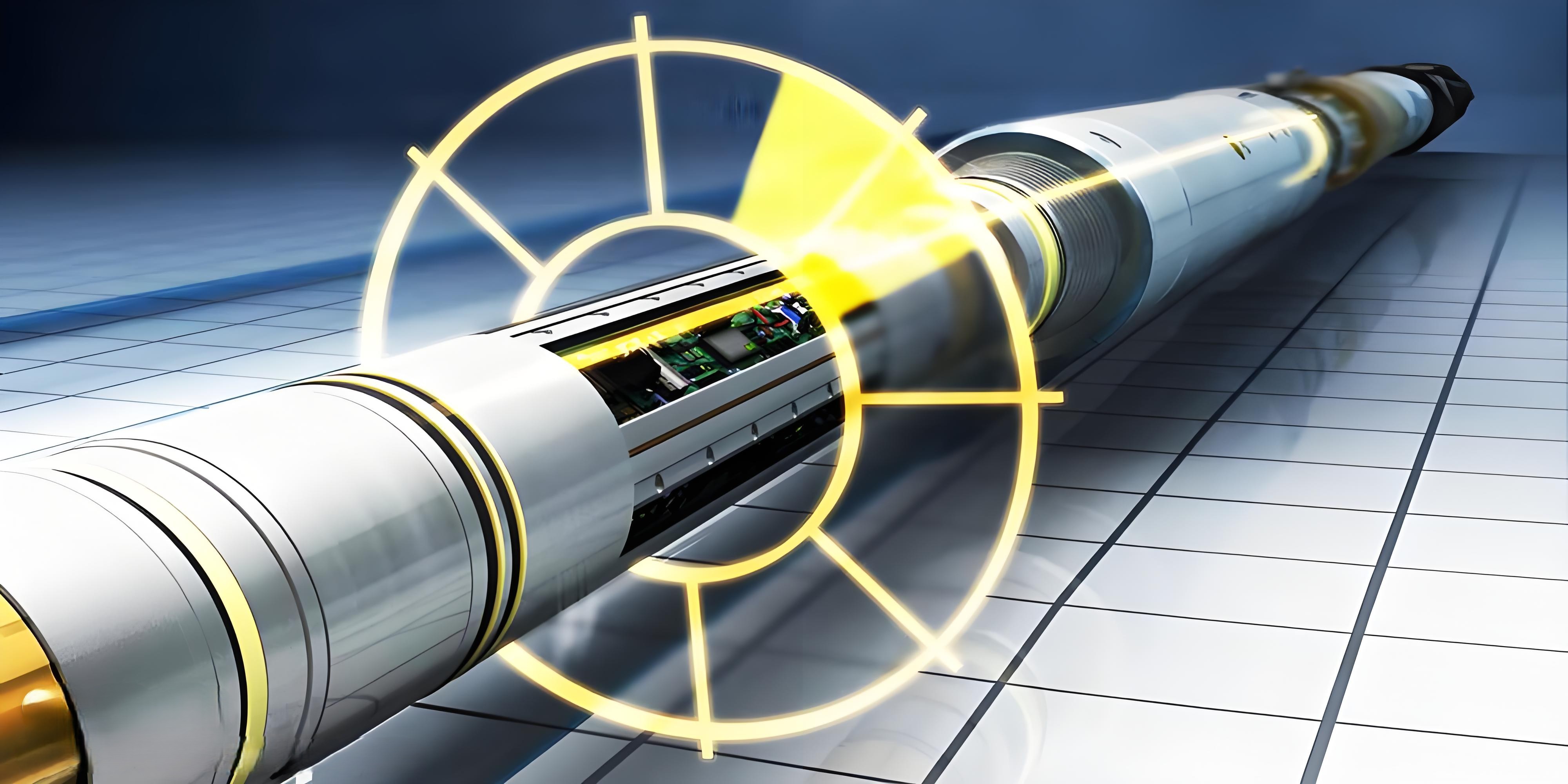
Hybrid control of drilling attitude
1. Introduction
In directional drilling, a downhole orientation tool enables trajectory steering by actuating a deflection mechanism to alter the borehole path 1,2. This process falls under drilling tool attitude control, and is a critical discipline involving direct manipulation of the bottom hole assembly (BHA) to orient the drill bit toward a target direction 3,4,5. Precise attitude control is, therefore, essential for accurate trajectory management 6,7. Fig. 1 illustrates the operational workflow of this control system, including real-time data transmission and directional adjustment.
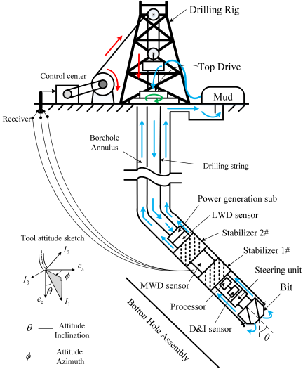
Fig. 1. Downhole drilling description.
The downhole drilling assembly comprises a drill string and a directional control system that integrates the BHA and the drill bit. The BHA, which is responsible for trajectory control, incorporates the following key components: a steering unit, a control module, direction and inclination (D\(\&\)I) sensors, stabilizers, and power-generation units 8,9. Critically, drill bit orientation is governed by the BHA’s attitude, making BHA posture the primary determinant of directional drilling accuracy 10,11.
The BHA attitude control module, which is integrated directly with the steering unit, comprises a central processing unit (CPU) and inertial measurement sensors 12,13. This module executes embedded control algorithms that (1) receive surface commands via mud-pulse telemetry, (2) process command parameters in real-time, and (3) generate actuation signals to manipulate the steering unit 14,15. Operational constraints including mud-pulse transmission latency (1.5–3 bit/s) and formation-induced signal attenuation necessitate real-time control algorithms to maintain attitude accuracy under dynamic downhole conditions.
Early attitude control research developed high-fidelity dynamic models that required full-state estimation 16,17. However, the computational complexity and inaccessibility of critical downhole state variables (e.g., instantaneous bit orientation) preclude their direct implementation in real-time control systems. Although these models have advanced the theoretical understanding of drilling tool mechanics, their practical utility remains limited by unmeasurable states and an excessive computational burden 18. To address this issue, Panchal et al. 16 derived a reduced-order dual-input–dual-output model using surface-measurable parameters and applied the small-gain theorem to rigorously analyze the feedback stability margins. Building on this foundation, a vector-based motion model was subsequently developed to characterize drilling tool dynamics under realistic downhole constraints 19.
Although Bayliss et al. 20,21 demonstrated significant progress in azimuth control methodologies, and other researchers advanced tool attitude optimization through refined control strategies 22,23, these approaches remain constrained by inherent limitations. Notably, they often assume linear dynamics, impose restrictive vector constraints, and treat azimuth control in isolation, neglecting the critical coupling between inclination and azimuth adjustments. To address these shortcomings, our work prioritizes kinematic model simplification and enhances control design feasibility. Specifically, we introduce a novel downhole feedback control system designed to compensate for nonlinear dynamics and borehole transmission delays, thereby enabling precise real-time orientation management of drilling tools.
The remainder of this study is structured as follows: Section 2 formulates the drilling tool motion model through attitude adjustment analysis; Section 3 presents the design of control system configuration and control problem description; Section 4 presents the theoretical framework and core control results; Section 5 validates the performance via simulation studies; and Section 6 concludes with an evaluation of inclination and azimuth control efficacy.
2. Drilling Attitude Adjustment and Model Establishment
2.1. Attitude Adjustment Description
Throughout the guided drilling operation, the system incorporates a comprehensive array of specialized components, including a drill bit, steering unit, processor, D\(\&\)I sensors, stabilizers, measurement-while-drilling (MWD) sensors, and power-supply devices, as illustrated in Fig. 1. The MWD sensor is designed to measure and record multiple drilling parameters, including, but not limited to, the drilling pressure, drilling rate, and other critical operational metrics. The MWD tool consists of two primary components: a surface-based signal receiver and a downhole signal transmitter integrated into the BHA. This configuration enables unidirectional data transmission from the subsurface to the surface, where the optimized signal transmission frequency contributes to enhanced communication efficiency and reduced power consumption of the MWD system. The D\(\&\)I sensor serves as the primary acquisition and processing unit for drill bit orientation data. The collected information is subsequently transmitted through the MWD module, which ultimately reaches the surface receiver for real-time monitoring and analysis.
The spatial orientation of the drilling tool is characterized by two fundamental parameters: inclination (\(\theta\)) and azimuth (\(\phi\)), whose geometric relationship and measurement principles are illustrated in Fig. 1. The inclination \(\theta\) quantitatively defines the vertical deviation of the drill bit advancement path from the vertical axis, whereas the azimuth \(\phi\) precisely characterizes the horizontal orientation of the drilling direction relative to true north. By establishing a mathematical correlation between these two angular parameters, the drilling tool motion is characterized using a mathematical model that enables precise control of the drilling process. This approach eliminates the dependence on complex downhole geometry parameters, enabling a simplified yet rigorous description of drilling tool dynamics.
The drilling trajectory is dynamically coupled to the drilling tool (i.e., the BHA) kinematics because the tool movement directly steers the trajectory path. Therefore, the three-dimensional spatial evolution of the drilling trajectory can be systematically determined and predicted. Consequently, attitude adjustment can be mathematically characterized as a functional relationship between inclination \(\theta\) and azimuth \(\phi\), which governs the spatial orientation of the drilling path.
2.2. Drilling Attitude Model
There are various types of directional drilling tools; however, push-type drilling tools use a controlled torque to steer the bit through rock layers and alter the drilling trajectory. In this study, a push-type drilling tool is selected as the primary research object. During drilling, the downhole tool rotates continuously, allowing it to be modeled as a rotating rigid body. To simplify the model, the lateral and torsional dynamic effects of the drill string and drilling tool assembly were not considered in the analysis. The dynamic equations for the system are as follows 16:
The dynamic equation presented above establishes the mathematical relationship between the drilling-tool-face angle \(\psi_{\mathrm{tf}}\), inclination \(\theta\), and azimuth \(\phi\). Furthermore, the two disturbance terms, \(H_{\mathrm{dr}}\) and \(H_{\mathrm{tr}}\), exhibit minimal influence and do not fundamentally alter the dynamic characteristics of the system. Consequently, these terms were neglected to simplify the model, yielding:
To facilitate subsequent system design and simplify its representation, the equivalent inputs are defined as follows:
3. Control System Design and Control Problem
3.1. Control System Configuration
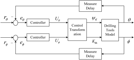
Fig. 2. The control system framework.
The architectural configuration of the attitude control system, as illustrated in Fig. 2, comprises two distinct control channels: one dedicated to regulating inclination \(\theta\) and another responsible for managing azimuth \(\phi\). The attitude control mechanism described herein represents a typical dual-channel control system that requires the integrated management of two coupled control parameters.
Notably, the output signals from both system controllers, represented as equivalent inputs \(U_{\theta}\) and \(U_{\phi}\), undergo a series of control transformations to be converted into the tool-face angle \(\psi_{\mathrm{tf}}\) and maximum curvatures \(K_{\mathrm{dls}}\) prior to their integration into the attitude control model. Moreover, the 20-meter physical distance between the D\(\&\)I sensor and steering tool in the BHA is a crucial factor. This spatial separation, coupled with the 5-bps pulse transmission rate, creates a non-negligible signal propagation delay that necessitates careful engineering considerations.
In the following sections, a comprehensive control formulation is presented, beginning with the architectural design of the inclination control loop and subsequently exploring the challenges inherent in the azimuth regulation mechanism.
3.2. Control Problem Formulation
The attitude control system integrates two distinct control loops: an inclination control loop and an azimuth control loop. Consequently, the formulation of the control problem is systematically addressed by examining both the inclination and azimuth aspects.
3.2.1. Attitude Inclination Control
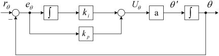
Fig. 3. Inclination control system.
Within the inclination control loop, a straightforward yet effective industrial proportional-integral (PI) control strategy is implemented in conjunction with the inclination differential equation. A schematic design of the inclination control loop is shown in Fig. 3. The dynamic equation governing the PI control of the inclination is presented as follows:
3.2.2. Attitude Azimuth Control
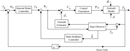
Fig. 4. Azimuth control system.
As illustrated in Fig. 4, the azimuth control system design exhibits greater complexity than its inclination counterpart. Substituting Eq. 4 into the framework yields the following state equation for the azimuth control:
Thus, the observer dynamics are given by:
The dynamic equation of the internal-model controller, derived in Fig. 4, is
The attitude azimuth estimate is then given by
The low-pass filter dynamics are governed by
The azimuth control loop exhibits stronger nonlinear coupling compared to the inclination control loop, necessitating specialized synthesis techniques for disturbance rejection.
4. Stability and Controller Design of Control System
Since the control loops for inclination \(\theta\) and azimuth \(\phi\) operate independently, their stability must be analyzed separately.
4.1. Attitude Inclination Correspondence
Based on Fig. 3, when the external input \(r_{\theta}\) is set to 0, the differential equations governing the inclination and its associated error are derived as follows:
The state-space equations for inclination dynamics are derived as
The characteristic equation governing inclination stability is \(\mathrm{det}(\lambda I - A_{\theta}) = 0\), where the symbol \(\lambda_{i}\) indicates the eigenvalue, and \(A_{\theta} \in \mathbb{R}^{n \times n}\):
4.2. Attitude Azimuth Correspondence
According to the separation theorem 24,25, the azimuth system decomposes into subsystem 1 (azimuth estimator and state observer) and subsystem 2 (internal-model controller, delay module, state-feedback controller, and azimuth model). With \(r_{\phi} = 0\) and \(d = 0\), the stability conditions of the two subsystems are analyzed separately.
Subsystem 1 utilizes a \(\gamma > 0\)-parameterized state-feedback controller:
The transfer function \(G_{e}(s)\) from \(\tilde{d}_{e}\) to \(\hat{d}_{e}\) is defined as follows:
For subsystem 2, introduce
Theorem 1: Given parameters \(\alpha\) and \(\beta\), the closed-loop system (Eq. 24) with the control law (Eq. 9) is asymptotically stable if symmetric positive definite matrices \(\mathcal{X}_{i}\), \(\mathcal{Y}_{i}\), \(\mathcal{M}_{i}\) (\(i =1, 2\)), and a matrix \(\mathcal{W}_{1}\) exist satisfying the following feasibility condition:
The gain of the state-feedback controller is as follows:
Proof 1: For the time-delay system under consideration, the Lyapunov–Krasovskii functional
Applying Jensen’s inequality 27, the derivative of the Lyapunov function satisfies
If \(\varPsi < 0\), then \(V'(\chi) < -\varepsilon\| \chi \|^{2}\) for \(\vee \varepsilon > 0\), which guarantees the asymptotic stability of system (Eq. 24). Applying the Schur-complement lemma to \(\varPsi < 0\) yields the equivalent linear matrix inequality (LMI):
Define the following block-diagonal transformations for \(i=1,\ 2\):
Applying a congruence transformation to LMI (Eq. 29) via the block-diagonal matrix diag\(\{\mathcal{X},\ \mathcal{X},\ \mathcal{M},\ \mathcal{X}\}\), using the transformations defined in Eq. 25 yields an equivalent LMI condition. Substituting the transformed system matrices \(\mathcal{A}\) and \(\mathcal{A}_{d}\) and eliminating the original dynamics matrices while preserving negative definiteness results in a tractable LMI formulation for convex optimization.
The certification process has been formally completed.
5. Case Study and Numerical Analysis
5.1. System Performance and Resource Savings
The control design efficacy was validated through a field case study using the push-type of BHAs. Tool-face orientation adjustments were executed in \(5{°}\) increments, extending the angular-correction time by 45%–55% relative to standard procedures (per ISO 13628-5 §6.2 compliance requirements).
\(H_{\mathrm{rop}}\) (150–250 ft/h) and \(K_{\mathrm{dls}}\) (\((6{°}\)–\(10{°})/100\) ft) dominate the system uncertainty for drilling-data analysis 28. Midpoint values (\(H_{\mathrm{rop}} = 200\)\(\pm\)50 ft/h, \(K_{\mathrm{dls}} = (8{°}\)\(2{°})/100\) ft) were selected to maintain operational safety margins while optimizing drilling efficiency within the established tolerances. All baseline parameters are summarized in Table 1.
Table 1. Simulation parameters.
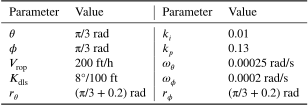
Table 1 lists the natural frequencies \(\omega_{\theta}\) (inclination control loop) and \(\omega_{\phi}\) (azimuth control loop), which serve as the critical stability parameters. These values define the operational bandwidth limits within which directional control systems maintain stability during rotary-steerable operations.
For the deviated inclination control, the PI gains are derived from 7,8 as \(k_{p} =\sqrt{2}\omega_{\theta}/a\) and \(k_{i}=\omega^{2}_{\theta}/a\), where parameter \(a\) is defined in Section 2.2. To ensure dimensional validity, expression \(a = H_{\mathrm{rop}}K_{\mathrm{dls}}\) is defined as the physical actuator time constant. The preceding analysis yielded \(k_{p} = 3.6665\), \(k_{i} = 0.0315\), and \(a = 7.755\times10^{-5}\) rad/s.
Subsequently, the azimuth control loop parameters were derived. The internal-model parameters are defined as
The observer gain \(L\) was synthesized via minimization of the performance index
5.2. Analysis of Attitude Adjustment Process
The tool attitude, defined by the inclination and azimuth, is kinematically controlled through the independent adjustment of these two angular parameters. This is analyzed here as a fundamental adjustment mechanism.
Based on the design constraints in Section 3.2.1 and field-engineering requirements, the inclination exhibits slow dynamics owing to the specific orientation characteristics of the drilling tool. Because derivative action in conventional PID control amplifies measurement noise and can destabilize slowly-varying trajectories, a PI control strategy is employed for inclination regulation.
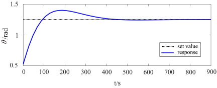
Fig. 5. Control response of attitude inclination.
Figure 5 shows that the inclination exhibits slow dynamics during the initial drilling phases, which is attributable to mud-pulse-telemetry-induced sensor delays. Provided that the ROP and DLS remain within operational bounds, the inclination stabilizes without the need for derivative action. The transient response settles within 6.0\(\pm\)0.3 minutes, aligning with durations documented in SPE field case studies (e.g., SPE 213456, 2022). These dynamics demonstrate a controlled, gradual convergence with minimal oscillation, achieving asymptotic stability within the quasi-steady operational regime.
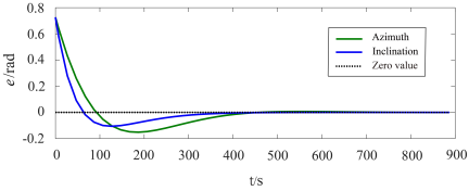
Fig. 6. Control error comparison of inclination and azimuth.
Figure 6 compares the transient error dynamics of the inclination and azimuth under PI control (a detailed analysis of the azimuth control performance under the PI strategy follows). The inclination control achieves a 22\(\%\) faster settling time and 28\(\%\) lower peak-error amplitude compared to the azimuth control, stabilizing within \(\pm\)0.2 rad steady-state tolerance. Consequently, the PI control of the inclination alone achieves a robust dynamic adjustment, eliminating the need for comparative PID implementations under these field constraints.
Adjusting the drilling tool orientation is inherently slow, and the resulting inclination changes align with actual field conditions. The attitude inclination control subsystem exhibits negligible overshoot and maintains stable performance with minimal fluctuations, thereby satisfying the practical engineering requirements for directional drilling applications.
Next, the performance of the azimuth control system is analyzed by introducing PI control as a baseline to evaluate the design effectiveness. Analogous to the inclination PI-controller design, the dynamic equation for the azimuth PI-controller takes the following form:
The azimuth dynamics are expressed by the following equation:
The state-space representation corresponding to Eq. 39 is given by
Similar to the derivation of the PI-gain parameters from the inclination, the proportional and integral gains of the azimuth control system are \(\overline{k}_{p} = \sqrt{2}\omega_{\phi}/(a\csc\theta)\) and \(\overline{k}_{i} = \omega^{2}_{\phi}/(a\csc\theta)\), respectively. Analysis of the data presented in Table 1, combined with the associated parameters, yields \(\overline{k}_{p} = 2.2877\) and \(\overline{k}_{i} = 0.0245\).
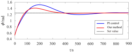
Fig. 7. Control response comparison for the azimuth.
The proposed method converges to a stable state in 350 s, representing a 48.5\(\%\) improvement over the 680 s required for the PI control (Fig. 7). Concurrently, peak oscillations are suppressed by 18\(\%\), demonstrating a significant performance enhancement in both transient and steady-state behaviors. These metrics confirm the superior performance of the proposed approach in terms of both response speed and stability.
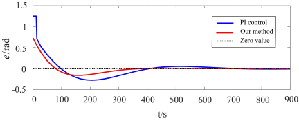
Fig. 8. Azimuth’s error comparison.
As shown in Fig. 8, the PI control struggles with initial error suppression owing to the nonlinear and delayed wellbore inclination dynamics. These factors generate destabilizing transients (delays and torque spikes) that jeopardize the integrity of the downhole tool. In contrast, the proposed method effectively bounds the inclination error within \(\pm\)0.2 rad, thereby eliminating excessive angular excursions and ensuring the structural integrity of the drilling assembly.
Compared to conventional PI control methodologies, the proposed method demonstrates superior performance in addressing the nonlinear dynamics and time delays inherent in azimuth regulation. Notably, the proposed control system exhibits a 48.5\(\%\) faster stabilization time than traditional PI implementations, significantly enhancing operational efficiency. This reduction in settling time and oscillation directly translates to reduced mechanical wear and an extended equipment lifespan.
The above analysis demonstrates that PI control leads to undesirable operational characteristics in azimuth regulation, including excessive response amplitude, increased structural stress on drilling tools, and prolonged stabilization times. These limitations collectively establish PI control as a suboptimal solution for high-precision applications, despite its eventual system stabilization.
6. Conclusion
This study presents an innovative control architecture for directional drilling, based on decoupled channels for the precise regulation of inclination and azimuth. For inclination control, the system utilizes a well-established PI control strategy, leveraging its proven stability and effectiveness in engineering applications. To address the more complex azimuth control requirements, a specialized feedback loop was engineered to counteract nonlinearities, measurement delays, and external disturbances (collectively termed as system interference). This hybrid approach effectively decouples the azimuth and inclination dynamics while mitigating delay-induced complexities.
Central to this hybrid design is the azimuth control module, which incorporates a dedicated azimuth estimator. This estimator significantly enhances the dynamic disturbance rejection capability of the loop. The gain of the state-feedback controller is rigorously determined using the LMI methodology to ensure optimal performance. Through these synergistic yet distinct control loops, the system achieves an efficient hybrid strategy for directional drilling tool orientation. The simulation results validate the effectiveness and robustness of this method, demonstrating marked improvements in the precision of the orientation-adjustment process.
This architecture excels in handling complex drilling dynamics while simultaneously catalyzing transformative advancements in drilling technology. By synergistically integrating proven control techniques with innovative feedback mechanisms, this design significantly enhances the precision, speed, and reliability of orientation control operations.
Acknowledgments
This work was supported by the Natural Science Foundation of Hubei Province, China, under Grant 2023AFB1003, and the Natural Science Foundation of Wuhan, China, under Grant 2024040801020341.
- [1] L. S. Jerez, E. Cayeux, and D. Sui, “Automatic calibration of systematic biases in directional drilling control for planar and non-planar curves,” Geoenergy Sci. Eng., Vol.246, Article No.213642, 2025. https://doi.org/10.1016/j.geoen.2024.213642
- [2] Z. Cai, X. Lai, M. Wu, L. Chen, and C. Lu, “Observer-based trajectory control for directional drilling process,” Asian J. Control., Vol.24, No.1, pp. 259-272, 2022. https://doi.org/10.1002/asjc.2456
- [3] K. Zhang and A. Huo, “Deep reinforcement learning attitude control of stabilized platform for rotary steerable system based on extended state observer,” J. Eng. Res., Vol.13, No.3, pp. 2777-2789, 2025. https://doi.org/10.1016/j.jer.2024.07.003
- [4] A. Huo, K. Zhang, and S. Zhang, “Attitude control of rotary steering drilling stabilized platform based on improved deep deterministic policy gradient,” SPE J., Vol.29, No.2, pp. 670-680, 2024. https://doi.org/10.2118/217992-PA
- [5] U. Zalluhoglu, J. Tilley, W. Zhang, and J. Grable, “Downhole attitude-hold controller leads to automatic steering of directional wells with improved accuracy and reduced tortuosity,” IADC/SPE Int. Drilling Conf. and Exhibition, Article No.SPE-199555-MS, 2020. https://doi.org/10.2118/199555-MS
- [6] D. Tian and X. Song, “Control of a directional downhole drilling system using a state barrier avoidance based method,” ASME. J. Dyn. Sys., Meas., Control., Vol.147, No.3, Article No.031005, 2025. https://doi.org/10.1115/1.4066454
- [7] A. Rehman, R. Ghias, I. Ahmad, and H. Iqbal Sherazi, “Advance optimized nonlinear control strategies for manage pressure drilling,” IEEE Access, Vol.12, pp. 73436-73450, 2024. https://doi.org/10.1109/ACCESS.2024.3404054
- [8] N. A. H. Kremers, E. Detournay, and N. van de Wouw, “Model-based robust control of directional drilling systems,” IEEE Trans. Control. Syst. Technol., Vol.24, No.1, pp. 226-239, 2016. https://doi.org/10.1109/tcst.2015.2427255
- [9] I. J. Isonguyo and J. F. Whidborne, “Bilinear modelling, control and stability of directional drilling,” Control. Eng. Pract., Vol.82, pp. 161-172, 2019. https://doi.org/10.1016/j.conengprac.2018.10.008
- [10] M. A. Faghihi, S. Tashakori, E. A. Yazdi, H. Mohammadi, M. Eghtesad, and N. van de Wouw, “Control of axial–torsional dynamics of a distributed drilling system,” IEEE Trans. Control. Syst. Technol., Vol.32, No.1, pp. 15-30, 2024. https://doi.org/10.1109/TCST.2023.3298255
- [11] A. Georgiou, S. A. Evangelou, I. M. Jaimoukha, and G. Downton, “Tracking control for directional drilling systems using robust feedback model predictive control,” IFAC-PapersOnLine, Vol.53, No.2, pp. 11974-11981, 2020. https://doi.org/10.1016/j.ifacol.2020.12.723
- [12] Z. Cai, X. Lai, M. Wu, C. Lu, and L. Chen, “Trajectory azimuth control based on equivalent input disturbance approach for directional drilling process,” J. Adv. Comput. Intell. Intell. Inform., Vol.25, No.1, pp. 31-39, 2021. https://doi.org/10.20965/jaciii.2021.p0031
- [13] Y. Yang, Y. Geng, J. Ye, and W. Wang, “Attitude estimation for drilling tools based on robust state-constrained zonotopic observer,” IEEE Sens. J., Vol.25, No.15, pp. 29064-29074, 2025. https://doi.org/10.1109/JSEN.2025.3580855
- [14] H. Yang, S. Gao, H. Liang, S. Luo, and P. Zhang, “Research on dynamic measurement method of drilling tool attitude near bit based on suppression of heavy-tailed measurement noise,” IEEE Sens. J., Vol.23, No.16, pp. 18384-18395, 2023. https://doi.org/10.1109/JSEN.2023.3289494
- [15] J. Tian, L. Mao, Y. Yang, H. Song, and J. Song, “Study on directional drilling coupling dynamics based on drill string rotary controller,” ASME J. Comput. Nonlinear. Dynam., Vol.18, No.9, Article No.091008, 2023. https://doi.org/10.1115/1.4062911
- [16] N. Panchal, M. T. Bayliss, and J. F. Whidborne, “Robust linear feedback control of attitude for directional drilling tools,” IFAC Proc. Volumes, Vol.43, No.9, pp. 92-97, 2010. https://doi.org/10.3182/20100802-3-ZA-2014.00022
- [17] M. Bayliss and J. Matheus, “Directional drilling tool simulation and system design,” SAE Int. J. Mater. Manuf., Vol.1, No.1, pp. 675-689, 2009. https://www.jstor.org/stable/26282704
- [18] G. C. Downton, “Challenges of modeling drilling systems for the purposes of automation and control,” IFAC Proc. Volumes, Vol.45, No.8, pp. 201-210, 2012. https://doi.org/10.3182/20120531-2-NO-4020.00054
- [19] N. Panchal, M. T. Bayliss, and J. Whidborne, “Attitude control system for directional drilling bottom hole assemblies,” IET Control. Theory Appl., Vol.6, No.7, pp. 884-892, 2012. https://doi.org/10.1049/iet-cta.2011.0438
- [20] M. T. Bayliss and J. F. Whidborne, “Mixed uncertainty analysis of pole placement and H∞ controllers for directional drilling attitude tracking,” J. Dyn. Sys., Meas., Control., Vol.137, No.12, Article No.121008, 2015. https://doi.org/10.1115/1.4031576
- [21] I. J. Inyang, J. F. Whidborne, and M. T. Bayliss, “Directional drilling attitude control with input disturbances and feedback delay,” IFAC-PapersOnLine, Vol.50, No.1, pp. 1409-1414, 2017. https://doi.org/10.1016/j.ifacol.2017.08.246
- [22] Z. Cai, X. Lai, M. Wu, C. Lu, and L. Chen, “Equivalent-input-disturbance-based robust control of drilling trajectory with weight-on-bit uncertainty in directional drilling,” ISA Trans., Vol.127, pp. 370-382, 2022. https://doi.org/10.1016/j.isatra.2021.08.032
- [23] M. V. Faronov and I. G. Polushin, “Observer-based control of vertical penetration rate in rotary drilling systems,” J. Process Control, Vol.106, pp. 29-43, 2021. https://doi.org/10.1016/j.jprocont.2021.08.016
- [24] J. Jiao, H. L. Trentelman, and M. K. Camlibel, “Distributed linear quadratic optimal control: compute locally and act globally,” IEEE Control. Syst. Lett., Vol.4, No.1, pp. 67-72, 2020. https://doi.org/10.1109/LCSYS.2019.2922189
- [25] P. Khargonekar, I. Petersen, and K. Zhou, “Robust stabilization of uncertain linear systems: quadratic stability and H_{infty} control theory,” IEEE Trans. Autom. Control., Vol.35, No.3, pp. 356-361, 1990. https://doi.org/10.1109/9.50357
- [26] H. Kimura, “A new approach to the perfect regulation and the bounded peaking in linear multivariable control systems,” IEEE Trans. Autom. Control., Vol.26, No.1, pp. 253-270, 1981. https://doi.org/10.1109/TAC.1981.1102573
- [27] K. Gu, “An integral inequality in the stability problem of time-delay systems,” Proc. of the 39th IEEE Conf. on Decision and Control, Vol.3, pp. 2805-2810, 2000. https://doi.org/10.1109/CDC.2000.914233
- [28] J. Kim and H. Myung, “Development of a novel hybrid-type rotary steerable system for directional drilling,” IEEE Access, Vol.5, pp. 24678-24687, 2017. https://doi.org/10.1109/ACCESS.2017.2768389
This article is published under a Creative Commons Attribution-NoDerivatives 4.0 Internationa License.