
Research Paper:
GSP-YOLO: An Efficient Tire Detection Algorithm for Truck Scale Scenarios
Qiaole Zhu, Quan Liang†, Nanlin Kuang, and Jinpeng Zhang
School of Computer Science and Mathematics, Fujian University of Technology
No.69 Xuefu South Road, Shangjie Town, Minhou County, Fuzhou, Fujian 350118, China
†Corresponding author

Truck scale systems are often located in complex industrial environments, and existing inspection methods based on the appearance of an entire vehicle are difficult to accurately locate trucks in space-constrained scenarios. This study proposes GSP-YOLO, a tire detection algorithm for truck scale scenarios based on an improved YOLOv8n, that assists in locating trucks on the scale by detecting tires and enhances the detection performance in industrial environments. GSP-YOLO incorporates a global-to-local spatial aggregation module into the neck structure to improve the perception of tires on small scales. A shared detail-enhanced convolutional detection head is designed in the detection head to enhance its ability to recognize complex features while reducing the computational cost. The model also replaces conventional convolution with poly-scale convolution to enhance object recognition capability and reduce feature loss. Additionally, the wise-intersection over union loss function is employed as the bounding box regression loss to suppress competition among high-quality anchors and reduce the impact of low-quality samples, thereby improving detection performance. The experimental results demonstrated that GSP-YOLO achieves an mAP50 of 89.3% on the dataset, representing a 2.0% improvement over the baseline model, and an increase of 0.9% in mAP50–95. This model significantly enhances the detection capability within truck scale systems and ensures reliable performance in complex industrial environments.
1. Introduction
Truck scale systems are widely used in industries such as logistics, mining, and construction to accurately measure the weight of vehicles. In traditional truck scale systems, devices such as photoelectric sensors and inductive loops are typically required to detect vehicle arrival and departure, thereby completing the weighing process. However, the deployment and maintenance of these devices incur high costs, and they are prone to malfunction owing to interference from external factors in complex environments. Therefore, new technologies are urgently required to replace traditional sensor-based methods for vehicle position detection at truck scales.
In recent years, deep learning-based object detection techniques have been widely applied in various industries. Current mainstream object detection algorithms are generally categorized into two types: two-stage and one-stage detection algorithms. The two-stage detection algorithm typically involves a region proposal stage followed by object classification and bounding box regression on the proposed regions. Representative algorithms in this category include the R-CNN 1, Fast R-CNN 2, Faster R-CNN 3, and Mask R-CNN 4. These methods demonstrate superior detection accuracy. However, their complex architectures and redundant computations result in slower inference speeds, making them less suitable for real-time applications. By contrast, one-stage detection algorithms eliminate the region proposal process and directly perform object localization and classification on the entire image. Notable examples include RetinaNet 5, the YOLO series 6,7,8,9,10,11, and SSD 12. These approaches significantly reduce computational complexity while maintaining acceptable accuracy, thereby improving detection efficiency and making them more suitable for real-time scenarios.
With the aid of computer vision, truck scale systems can utilize cameras to detect and locate the positions of trucks on the scale, thereby replacing the expensive sensor equipment used in traditional methods. Furthermore, cameras are easier to install and maintain than sensors. However, to capture the full view of both the truck and scale, particularly for long truck scales, cameras typically need to be placed at a sufficiently high and distant location. Confined industrial environments often have insufficient space for camera installation. Consequently, vehicle positioning based on tire feature detection has emerged as a viable alternative. This approach reduces the distance requirements for camera deployment and is better suited for installation in narrow spaces. Nevertheless, the complex environmental factors commonly observed in industrial settings, such as dust pollution, lighting variations, and interference from rain or fog, still pose significant challenges to the robustness of detection algorithms. Therefore, this study proposes an improved model based on YOLOv8n, named GSP-YOLO, aimed at enhancing tire detection performance in truck scale scenarios. The main contributions of this study are as follows:
-
(1)
Because tires appear as small-scale targets at long distances from the camera and are easily confused with the background, the global-to-local spatial aggregation (GLSA) module 13 was introduced into the neck network to simultaneously fuse global context and local detailed features, thereby enhancing the ability of the model to localize tire targets and discriminate them from complex backgrounds, particularly for small-scale tires.
-
(2)
Repeated convolution operations in the detection head can lead to computational redundancy and complicate the full capture of fine-grained features. In the detection head module, a shared detail-enhanced convolutional detection head (SDEHead) was proposed to reduce the computational complexity of the model while enhancing the ability of the detection head to recognize complex features.
-
(3)
When trucks enter a weighbridge, the tire targets exhibit significant scale variations. To address this, the poly-scale convolution (PSConv) module 14 was introduced that improved the adaptability and robustness of the model to target scale variations without adding extra parameters or increasing the computational cost.
-
(4)
In industrial weighbridge scenarios, low-quality anchor samples can negatively affect gradient updates. To address this, the wise-intersection over union (WIoU) loss function 15 was incorporated into the loss design, using a dynamic non-monotonic focusing mechanism and a gradient gain allocation strategy to mitigate the adverse effects of low-quality samples, thereby improving the convergence speed and bounding box regression accuracy of the model.
Through the synergistic optimization of GLSA, SDEHead, PSConv, and WIoU, the overall performance of GSP-YOLO is significantly improved. GLSA provided fused global and local spatial information to enhance the localization of small-scale tires, SDEHead improved the computational efficiency of the detection head and its ability to recognize complex features, PSConv strengthened the adaptability and robustness of the model to tires of varying scales, and WIoU enhanced the stability and accuracy of bounding box regression. This coordinated design significantly improved the capability and reliability of tire detection in truck scale scenarios.
2. Related Works
2.1. YOLOv8
YOLOv8 is an improved model developed by the Ultralytics team based on the YOLOv5 architecture. The model is divided into five different scales, n, s, m, l, and x, according to the network depth. The architecture of YOLOv8 comprises three main components: backbone, neck, and detection head.
The backbone primarily comprises CBS, C2f feature extraction, and spatial pyramid pooling-fast (SPPF) modules. The CBS module integrates convolution, batch normalization, and the SiLU activation function. The C2f module, a specialized component in YOLOv8n, replaces the traditional C3 module and enhances gradient propagation efficiency. The SPPF module is an optimized version of the original SPP module 16, designed to expand the receptive field. The neck network adopts the feature pyramid network 17 and path aggregation network 18 to collaboratively process multi-scale feature maps, enhancing the semantic information interaction between the upper and lower layers. This effectively improves the representation of object features and alleviates the problem of vanishing gradients in deep networks. The detection head uses a decoupled structure to separately optimize classification and regression tasks, thereby improving the generalization capability of the model.
2.2. Wheel Detection
In recent years, computer vision technology has been widely applied in various fields such as transportation, healthcare, and bioinformatics. In the field of wheel detection, researchers have proposed various methods to improve detection accuracy and robustness under complex scenarios. Li et al. 19 addressed the limited accuracy of the traditional Hough transform in circular object detection by proposing a wheel detection method based on HOG features and an SVM classifier that extracted edge features and performed training and recognition using an SVM. OBrien et al. 20 designed a method that combines a magnified circular pseudo-wavelet filter with a circularity-weighted detection algorithm, improving detection performance under varying lighting conditions. Another class of methods integrated multiple feature extraction techniques. For example, Ruan et al. 21 constructed a precise wheel detector by combining HOG and MB-LBP features with an AdaBoost classifier, enabling the accurate localization and recognition of wheels. Ghanem and Kerekes 22 trained an SSD model to precisely extract wheel bounding boxes and discriminative features from full-vehicle images that was applied to vehicle re-identification tasks. Shenoda 23 proposed a real-time wheel detection algorithm based on YOLOv5 to specifically address the detection challenges caused by camera angles, lighting variation, and complex environments.
Despite the significant progress achieved by the aforementioned methods in the field of wheel detection, certain limitations remain when addressing challenges in real-world industrial environments. In particular, under harsh conditions such as severe dust pollution and drastic lighting variations, ensuring stable and accurate detection is often difficult; this restricts their effectiveness in practical applications such as truck scale systems.
3. Research Methods
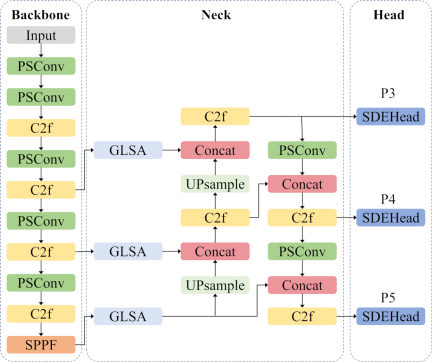
Fig. 1. Network structure of GSP-YOLO.
To satisfy real-time tire detection requirements in truck scale scenarios, this study focuses on resource-constrained industrial edge devices and environments, with priority given to computational efficiency and deployment adaptability. Based on a comparative analysis of YOLOv8 architectures, YOLOv8n offers lower computational complexity and memory usage, making it better suited for real-time processing on edge devices. Therefore, YOLOv8n is selected as the base architecture in this study to ensure efficient operation under limited computational resources.
PSConv is introduced to replace the standard convolutional modules in the network, and a GLSA structure is incorporated into the neck. The detection head employs the SDEHead module, and WIoU is adopted in place of CIoU as the loss function for the bounding box regression. The architecture of the improved model, GSP-YOLO, is illustrated in Fig. 1.
3.1. Global-to-Local Spatial Aggregation Module
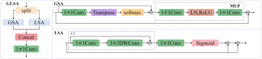
Fig. 2. Architecture of the GLSA module.
YOLOv8 faces certain limitations when handling objects at different scales, particularly in truck scale scenarios in which tire targets are often extremely small before the truck approaches the scale, leading to decreased detection accuracy. Although high-level features provide a global context, they tend to overlook the fine details of small objects. Conversely, low-level features contain rich local information but struggle to effectively capture the overall semantics. Additionally, in complex scenes with occlusions or lighting variations, high-level features are prone to false positives, reducing the ability of the model to distinguish between the targets and background. To address these issues, the GLSA module 13 is introduced, enabling better fusion of global and local information, enhancing localization of targets, and improving generalization performance in challenging environments. The structural diagram of the GLSA module is shown in Fig. 2.
The GLSA module optimizes high-level feature representations by aggregating multi-scale spatial features from global to local, thus reducing the false positive rate in high-level features. This module comprises two submodules: local spatial attention (LSA) and global spatial attention (GSA). The LSA submodule focuses on enhancing the fine-grained feature description of small-scale targets, thereby effectively addressing challenges such as local feature loss and the difficulty in detecting small tire targets. The GSA submodule captures and integrates global contextual information to strengthen the ability of the model to distinguish foreground objects from background environments, thereby improving the generalization performance in complex scenarios involving occlusions, lighting variations, and other challenging conditions. The GLSA module evenly divides input feature \(F_{i} \in \mathbb{R}^{C \times H \times W}\) along the channel dimension into \(F_{i}^{1}, F_{i}^{2} \in \mathbb{R}^{(C/2) \times H \times W}\), that are separately fed into the GSA and LSA modules. The outputs of the two paths are concatenated and connected through a \(1 \times 1\) convolutional layer. The detailed module structure is described by Eqs. 1 and 2.
3.1.1. GSA Module
The purpose of the GSA module is to capture the long-range spatial dependencies of each pixel, thereby supplementing the missing global contextual information in local features. The computation of GSA is given by Eqs. 3 and 4.
Here, \(\mathit{Att}_{G}(\cdot)\) denotes the attention operation and \(C_{1\times 1}\) represents a \(1 \times 1\) convolution. \(\mathrm{Transpose}(\cdot)\) denotes the transpose operation that is used to rearrange the order of feature dimensions to enable the computation of attention weights at a global scale. Matrix multiplication is performed using operator \(\otimes\). \(\mathit{MLP}(\cdot)\) comprises two dense layers, and ReLU activation and normalization are applied between them. In the MLP, the first layer expands the input dimension by an expansion ratio of two, enhancing the representation capacity of the network to learn more complex features, and the second layer projects the features back to the original dimensionality.
3.1.2. LSA Module
The purpose of the LSA module is to effectively extract local features from regions of interest along the spatial dimensions of a given feature map, such as small objects in the image. The LSA computation is given in Eqs. 5 and 6.
\(F_{c}(\cdot)\) denotes a cascade of three \(1 \times 1\) convolutional layers followed by a \(3 \times 3\) depthwise convolutional layer. \(\mathit{Att}_{L}(\cdot)\) defines the local attention operation. \(\sigma(\cdot)\) and \(\odot\) denote the sigmoid activation function and element-wise multiplication, respectively. This design facilitates the effective integration of local spatial cues while maintaining a compact parameter footprint.
3.2. Shared Detail-Enhanced Convolutional Detection Head
The detection head of YOLOv8 adopts a decoupled structural design in which separate branches, each composed of two \(3 \times 3\) convolutional layers followed by a \(1 \times 1\) convolutional layer, are used to extract classification and localization features. However, this architecture presents certain limitations. First, each detection head performs identical convolutional operations, resulting in parameter redundancy and repeated computations that increase model complexity and constrain inference efficiency in scenarios with limited resources. Second, the decoupled design leads to the independent processing of input features across detection heads, lacking interaction between feature maps and limiting the ability of the model to effectively capture features in complex backgrounds. Considering the real-time detection requirements in truck scale localization scenarios, as well as the fact that images in industrial truck scale applications are often affected by dust, weather changes, and other environmental factors that weaken the feature information in the tire regions and lead to degraded image quality, this study proposes a novel shared convolution detection head, SDEHead. The architecture of the SDEHead module is illustrated in Fig. 3. The design methodology is as follows:
-
(1)
Weight-Sharing Mechanism: A convolutional weight-sharing mechanism is employed to fuse multi-scale feature maps from the neck of the YOLOv8 model. This mechanism significantly reduces the number of trainable parameters and the computational cost, thereby enhancing computational efficiency and reducing the risk of overfitting.
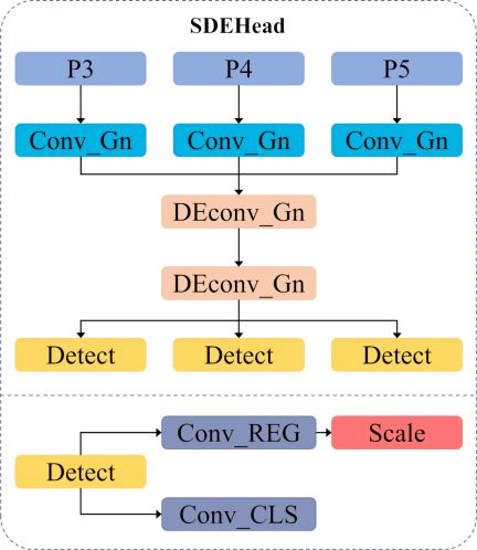
Fig. 3. Architecture of the SDEHead module.
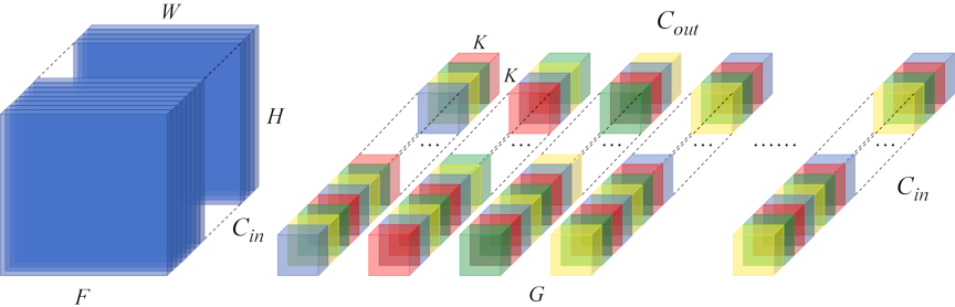
Fig. 4. PSConv schematic.
-
(2)
Enhanced Feature Extraction using DEConv: Although shared convolution reduces the computational cost and parameter count of the model, it is insufficient for capturing complex details. To address this issue, SDEHead incorporates a detail-enhanced convolution (DEConv) 24 that extracts richer feature information from multiple directions and perspectives. DEConv comprises four differential convolutions and one standard convolution. The four differential convolutions include center difference convolution (CDC), angular difference convolution (ADC), horizontal difference convolution (HDC), and vertical difference convolution (VDC). The CDC emphasizes local relative changes by computing the differences between the central pixel and its neighboring pixels, highlighting subtle texture variations and allowing the model to preserve discriminative tire surface details under conditions such as dust coverage or slight blurring. HDC and VDC extract gradient features along the horizontal and vertical directions, respectively, thereby strengthening the representation of the main tire edges and enhancing the stability of feature representations for key tire contours under complex imaging conditions. ADC captures oblique texture variations, compensates for details that cannot be covered by HDC and VDC, and enhances the ability of the model to recognize angled textures. Through the collaborative effect of these four difference convolutions, SDEHead maintains stable representations of tire edges and texture features under challenging industrial conditions, such as dust- and weather-induced image degradation, thereby significantly improving the ability and robustness of the detection head in recognizing complex target features.
-
(3)
Group Normalization for Efficient Inference: Group normalization 25 is adopted to replace the traditional batch normalization. Batch normalization relies on sufficiently large batch sizes to maintain stable performance, a practice that can degrade performance under limited conditions and often leads to memory bottlenecks during large-scale processing. By contrast, group normalization divides all channels into groups and computes the mean and variance within each group for normalization. This allows for efficient training even with small batch sizes, significantly reducing hardware requirements and the dependency on batch size, which in turn improve the inference efficiency of the model.
3.3. Poly-Scale Convolution
In traditional convolutional neural networks, the kernel size is typically fixed. However, in real-world applications, the objects in feature maps often vary significantly in scale and shape. Fixed-size kernels may fail to effectively capture the features of targets with diverse sizes, thereby limiting the ability of the model to perceive and represent multi-scale objects. Existing research commonly focuses on extracting multi-scale features through layer- or filter-wise strategies, emphasizing the overall network architecture. By contrast, PSConv 14 addresses this limitation from a finer-grained perspective at the kernel level, shifting the design focus from macro-level structures to micro-level modules. This enables the efficient utilization of multi-scale features without altering the overall network structure.
PSConv follows two core design principles. First, each convolutional filter uses a set of dilation rates within its kernel to extract the features across different receptive fields. Second, for all the convolutional filters within a single layer, the combinations of dilation rates are cyclically alternated across the input and output channels, allowing the network to capture multi-scale information from the input and effectively map it to the output features. A schematic of the PSConv mechanism is presented in Fig. 4.
Let the input feature map be denoted as \(F \in \mathbb{R}^{C_{\mathit{in}} \times H \times W}\) and the output feature map as \(H \in \mathbb{R}^{C_{\mathit{out}} \times H \times W}\), where \(C_{\mathit{in}}\) represents the number of input channels, \(H\) and \(W\) denote the height and width of the feature maps, respectively, and \(C_{\mathit{out}}\) denotes the number of output channels. The convolution kernel is represented as \(G \in \mathbb{R}^{C_{\mathit{out}} \times C_{\mathit{in}} \times K \times K}\). The computation of a standard convolution at spatial position \((x, y)\) for the \(c\)-th output channel can be expressed as follows:
Here, \(c \in \{1, \ldots, C_{\mathit{out}}\}\) and \(k \in \{1, \ldots, C_{\mathit{in}}\}\) denote the indices of the output and input channels, respectively. \(x\) and \(y\) denote the spatial location indices in the feature map, where \(x \in \{1, \ldots, H\}\) and \(y \in \{1, \ldots, W\}\). \(i\) and \(j\) represent the relative spatial offsets of the convolution kernel centered at location \((x, y)\). \(G_{c, k, i, j}\) denotes the corresponding convolution kernel weight, and \(F_{k, x+i, y+j}\) denotes the feature value of the input feature map at the specified channel and spatial location.
PSConv assigns different dilation rates to distinct convolution kernels within a single convolutional filter in an organized manner, enabling features to simultaneously capture spatial contextual information at multiple scales. This design fully exploits the multi-scale modeling capability of dilated convolutions without introducing additional computational overhead. Moreover, cross-channel representations at multiple spatial scales are aggregated through a linearly weighted summation, while allowing each individual input channel to extract features under multiple receptive fields. The formulation of PSConv is given in Eq. 8.
\(D \in \mathbb{R}^{C_{\mathit{out}} \times C_{\mathit{in}}}\) denotes the matrix of the dilation rates. Specifically, each entry \(D_{(c,k)}\) is mapped to a particular channel within a given filter that assigns a distinct dilation rate to the corresponding convolution kernel, \(G_{c,k,\cdot,\cdot}\). By introducing the PSConv module, this study periodically configures differentiated dilation rate matrices across channels and filters to achieve cross-scale feature fusion within a single convolution without adding extra parameters or increasing computational complexity, thereby enhancing the feature extraction capability for tire detection in complex industrial scenarios.
3.4. WIoU Loss Function
YOLOv8 originally used CIoU 26 as the loss function for bounding box regression. Nevertheless, the CIoU exhibits a higher sensitivity to high-quality samples, whereas low-quality samples yield weaker gradients, limiting their contribution to the optimization process. Consequently, the model tends to focus on easy-to-learn samples during training. This becomes a limitation in tire detection tasks, particularly under challenging conditions such as uneven lighting or severe weather in which the image quality often fluctuates and the model struggles to learn effective information from low-quality samples, ultimately affecting the detection accuracy.
To address this issue, the V3 variant of the WIoU 15 formulation is adopted as the loss function for the bounding box regression. WIoUv3 employs a dynamic non-monotonic focusing mechanism to evaluate the anchor box quality through an outlier degree metric. Additionally, it incorporates a gradient gain allocation strategy that effectively suppresses excessive competition among high-quality anchors and mitigates the negative gradient impact of low-quality examples. These enhancements improve the stability and overall performance of the detector. The computation of the WIoU is shown in Eqs. 9 and 10.
Here, \((x, y)\) and \((x_{gt}, y_{gt})\) denote the center coordinates of the predicted and ground-truth bounding boxes, respectively. \(W_{g}\) and \(H_{g}\) represent the width and height, respectively, of the minimum enclosing rectangle covering both boxes. \(R_{\mathit{WIoU}} \in [1, e)\) is introduced to strengthen the \(L_{\mathit{IoU}}\) contribution for normal-quality anchor boxes. \(L_{\mathit{IoU}} \in [0, 1]\) markedly decreases the \(R_{\mathit{WIoU}}\) value of high-quality anchor boxes and shifts the optimization focus toward the distance between the center points when the anchor box closely matches the target box. Symbol \(*\) denotes a detach operation in which \(W_{g}\) and \(H_{g}\) are excluded from backpropagation to prevent \(R_{\mathit{WIoU}}\) from adversely affecting model convergence.
\(\beta \in [0, +\infty)\) is defined as the outlier degree to measure the quality of anchor boxes, and the formulation is given as follows:
\(L^{*}_{\mathit{IoU}}\) denotes a monotonic focusing coefficient and \(\overline{L_{\mathit{IoU}}}\) represents its mean value that varies with \(L_{\mathit{IoU}}\). A smaller \(\beta\) indicates a high-quality anchor box, whereas a larger \(\beta\) corresponds to a low-quality anchor box. Both are assigned reduced gradient gains, thereby guiding bounding box regression to focus on normal-quality samples while mitigating adverse gradient effects caused by low-quality anchors. A non-monotonic focusing coefficient \(r\) is constructed based on \(\beta\), and the formulation of WIoUv3 is given as follows:
\(\alpha\) and \(\delta\) are hyperparameters. The dynamic \(\overline{L_{\mathit{IoU}}}\) adaptively partitions the anchor box quality levels, enabling WIoUv3 to reasonably adjust gradient gain allocation, thereby enhancing the learning capability and detection accuracy of the model for different tire targets.
4. Experimental Procedure Design
4.1. Experimental Datasets
The dataset used in this study primarily comprised publicly available datasets and real-world tire images captured onsite at a truck scale station using surveillance cameras. The public datasets included images collected from various websites on the Internet and selected images from the Open Images V7 public dataset. During the selection of publicly available datasets, images with diverse vehicle characteristics, environmental backgrounds, and weather conditions were selected to enhance dataset diversity.
For real-world scenarios, tire images were collected from a truck scale system in an operational industrial park. The data collection process was conducted without affecting the normal factory operations to ensure that the data accurately reflect the actual industrial environment. The specific data acquisition procedure is as follows:
-
(1)
Cameras were installed at two diagonal positions of the truck scale, with their heights adjusted appropriately to ensure that the field of view covered both the scale area and truck tires during vehicle entry.
-
(2)
Images were captured at different key stages of the trucks passing over the scale, including the initial entry, during weighing, while moving on the scale, and before leaving the scale, thereby obtaining samples with diverse tire poses and motion states.
-
(3)
Data were collected under various environmental conditions, including daytime and nighttime scenes and under different weather conditions such as sunny and rainy, to enhance the diversity and robustness of the dataset in real industrial environments.
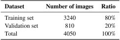
The dataset was split into training and validation sets with a ratio of \(8 \mathbin{:} 2\). The training set was used to learn the model parameters, whereas the validation set is employed to evaluate the model performance. The detailed statistics of the dataset are presented in Table 1. The input data must be standardized before use to satisfy the requirements of different deep learning networks. In this study, the wheel objects in the images were manually annotated using the LabelImg dataset labeling tool. The annotations followed the VOC format and included the normalized coordinates of each target center point, along with the width and height of the corresponding bounding box.
Table 1. Dataset split statistics.
4.2. Evaluation Metrics
To evaluate and compare the performance of the models, this study uses precision (P), recall (R), floating point operations (FLOPs), mAP50, and mAP50–95 as the evaluation metrics. The formulas for calculating P, R, and mAP are as follows:
\(\mathit{TP}\) represents true positives, indicating the number of positive samples correctly identified as positive. \(\mathit{FP}\) represents false positives, indicating the number of negative samples incorrectly identified as positive. \(\mathit{FN}\) represents false negatives, indicating the number of positive samples incorrectly identified as negative. \(n\) denotes the total number of classes in the dataset. The FLOPs are metrics used to measure the computational cost of a model during inference. It represents the number of FLOPs and is used to assess the computational complexity and efficiency of the model.
4.3. Experimental Environment
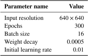
The experiments were conducted on a Windows 11 operating system with an NVIDIA GeForce RTX 4060 GPU, and a 13th Gen Intel® Core™ i9-13900HX CPU, using the PyTorch 2.1.2 deep learning framework and CUDA 12.1. The experimental parameter settings are listed in Table 2.
Table 2. Parameters of the experiment.
5. Experimental Results and Analyses
5.1. Comparison Experiments of Different Detection Heads
To verify the effectiveness of the SDEHead detection head module, this study applied SDEHead, DyHead 27, SEAMHead 28, MultiSEAMHead, and EfficientHead to the same YOLOv8n baseline model for comparison. The detection performances were analyzed and compared. The results are summarized in Table 3.
Table 3. Comparison results of different detection heads.
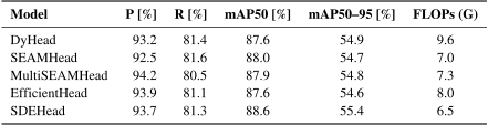
The results showed that significant differences existed in the detection performance and computational complexity among the various detection head modules. DyHead achieved an mAP50 of 87.6% but suffered from a relatively large FLOPs of 9.6G. SEAMHead reduced FLOPs to 7.0G while achieving a recall of 81.6% and an mAP50 of 88.0%; however, its precision showed a noticeable decline compared with other methods. MultiSEAMHead further improved the precision to 94.2%, although the recall slightly dropped to 80.5%, and FLOPs slightly increased to 7.3G. While this enhanced the detection accuracy, it sacrificed part of the recall performance. EfficientHead exhibited relatively high FLOPs of 8.0G, second only to DyHead, and its detection performance showed no significant advantage compared with other methods. The SDEHead detection head achieved the highest mAP50 and mAP50–95 among all compared detection heads, reaching 88.6% and 55.4%, respectively, while reducing FLOPs to the lowest among all compared methods, at only 6.5G, effectively demonstrating its advantage in improving detection performance while minimizing computational complexity.
5.2. Comparison Experiments of Different Loss Functions
In response to the uneven contribution of low-quality bounding boxes to the regression loss during the CIoU training process, experiments were conducted using a baseline model to evaluate the performances of WIoU, CIoU, DIoU 29, SIoU 30, and GIoU 31. The results are summarized in Table 4.
Table 4. Comparison results of different loss functions.
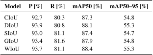
The experimental results demonstrated that the WIoU loss function delivered the best performance, particularly achieving the highest mAP50 value of 88.4%, significantly outperforming other methods and indicating superior object localization accuracy. Moreover, WIoU achieved the highest score on the mAP50–95 metric, reaching 55.3%, equally matched by DIoU and surpassing 54.8% of CIoU. In terms of precision, WIoU reached 93.7%, second only to 93.9% of DIoU; for recall, WIoU achieved 81.1%, showing an improvement over CIoU. Considering all metrics, WIoU demonstrated a well-balanced performance by ensuring detection accuracy while maintaining stability and robustness, thereby validating its effectiveness as a bounding box regression loss function and showcasing its superior overall capability.
5.3. Ablation Experiments
To systematically evaluate the contribution of each optimization strategy to the object detection system, this study employed an ablation experimental design to quantify the impact of each improvement module on the model performance. A “\(\checkmark\)” indicates the module was used, whereas a “\(\times\)” indicates it was not. The experimental results are listed in Table 5.
Table 5. Results of the ablation experiment.
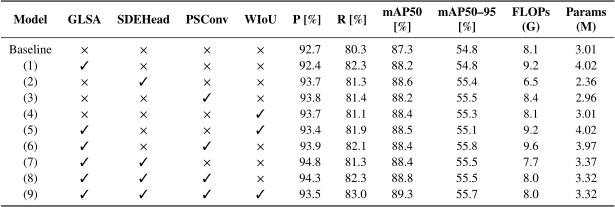
Table 6. Comparison results of different models.
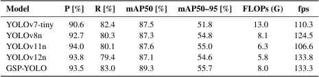
Table 5 presents the ablation study results obtained by progressively introducing different modules into the YOLOv8n baseline, and further quantifies the impact of each module on the detection performance, computational complexity, and parameter scale.
First, a comparison of the baseline results model with those of Model (1) showed the introduction of GLSA increased the FLOPs from 8.1G to 9.2G, whereas the number of parameters increased from 3.01M to 4.02M. This increase mainly originated from the GSA branch of GLSA that established attention relationships over the entire spatial domain. Although the GSA operated on feature representations with halved channel dimensions, its attention computation still involved modeling global dependencies among all spatial locations and aggregating features through matrix operations between attention weights and feature maps. When applied to high-resolution feature maps, these large-scale spatial-level computations significantly amplified the overall FLOPs, resulting in higher computational overhead. Despite this increase in computation and parameters, GLSA effectively enhanced the ability of the model to localize tire targets and distinguish them from complex backgrounds by jointly integrating global contextual information and local details, leading to an improvement in recall from 80.3% to 82.3% and an increase in mAP50 to 88.2%.
To further analyze the individual contribution of each module, Models (2)–(4) independently introduced SDEHead, PSConv, and WIoU into the baseline model. A comparison of the experimental results with those of the baseline model showed SDEHead significantly reduced the parameter count to 2.36M and FLOPs to 6.5G, while simultaneously improving precision, recall, and mAP. This indicated that, through convolutional weight sharing and detail-enhanced convolutional structures, SDEHead effectively reduced the number of trainable parameters and the computational burden while improving detection performance. PSConv achieved improvements across all evaluation metrics with only a slight increase in FLOPs compared with the baseline model. WIoU maintained the same computational complexity and parameter count while still contributing to stable improvements in detection accuracy.
Models (5) and (6) further investigated the combined effects of GLSA with WIoU and PSConv, respectively. Incorporating WIoU alongside GLSA improved the mAP without introducing additional computational costs. In contrast, combining GLSA with PSConv increased the FLOPs to 9.6G, with a parameter count of 3.97M. Compared with Model (3) that introduced only PSConv, the incorporation of GLSA caused additional computational overhead owing to the GSA branch, indicating that GLSA remained the primary source of increased computational complexity.
Notably, when GLSA and SDEHead were jointly introduced in Model (7), the FLOPs were significantly reduced from 9.2G to 7.7G compared with Model (1), whereas the precision improved to 94.8% and the mAP50–95 reached 55.5%. This demonstrated that SDEHead could effectively compensate for the computational overhead introduced by the GSA branch within GLSA, optimizing the overall efficiency while further enhancing the detection accuracy.
Finally, Model (9), that simultaneously integrated GLSA, SDEHead, PSConv, and WIoU, achieved the best overall performance with only 8.0G FLOPs and 3.32M parameters. Specifically, the recall and mAP50 reached 83.0% and 89.3%, respectively, representing improvements of 2.7% and 2.0% over the baseline, respectively, and achieving the best performance among all the evaluated models. The precision was further improved compared with the baseline, reaching 93.5%. The mAP50–95 attained 55.7%; this was only slightly lower than that of Model (6) that achieved 55.8%. Overall, the analysis indicated that GLSA enhanced the capability of the model to localize small targets and discriminate foreground objects from complex backgrounds at the cost of increased computation; SDEHead significantly reduced the computational complexity and parameter overhead introduced by GLSA through convolutional weight sharing while improving accuracy; PSConv balanced performance gains with computational efficiency; and WIoU further refined regression quality without increasing inference cost. The modules complemented each other in terms of performance improvement and computational efficiency, allowing the final model to achieve a favorable balance between accuracy and efficiency while maintaining a computational complexity and parameter count comparable to those of the baseline.
5.4. Comparison Experiments with Different Models
Representative YOLO series models were selected for comparison with the GSP-YOLO model to evaluate the detection accuracy and real-time performance of the proposed model. All the models were evaluated under the same experimental environment and testing conditions, as described in Section 4.3, and the results are presented in Table 6.
As presented in Table 6, the GSP-YOLO model achieved the highest recall, mAP50, and mAP50–95, reaching 83.0%, 89.3%, and 55.7%, respectively, outperforming all the compared models. In terms of precision, GSP-YOLO reached 93.5%, showing improvements over YOLOv7-tiny and YOLOv8n. Although its precision was slightly lower than those of YOLOv11n and YOLOv12n, GSP-YOLO maintained superior performance in terms of the recall and mAP metrics. Regarding computational complexity, the FLOPs of GSP-YOLO were 8.0G; this was considerably lower than 13.0G of YOLOv7-tiny and slightly lower than 8.1G of YOLOv8n. Although it was marginally higher than those of YOLOv11n and YOLOv12n, GSP-YOLO achieved better detection accuracy while maintaining a relatively low computational cost. In terms of real-time performance, GSP-YOLO achieved an inference speed of 133.3 fps that was significantly higher than those of YOLOv7-tiny, YOLOv8n, and YOLOv11n, and only slightly lower than that of YOLOv12n, indicating that the proposed model did not significantly sacrifice inference speed while improving detection accuracy. Therefore, GSP-YOLO effectively balanced the detection accuracy, recall, computational complexity, and real-time performance, demonstrating a strong overall detection capability and promising potential for practical applications.
5.5. Visual Analysis
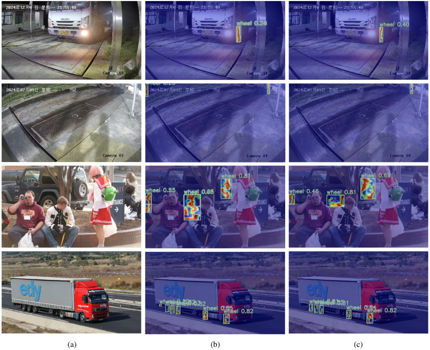
Fig. 5. Comparison of heatmap detection results. (a) Original images; (b) YOLOv8n; and (c) GSP-YOLO.
To more intuitively demonstrate the performance of the proposed improved model in object detection tasks, the HiResCAM 32 heatmap visualization method was employed to analyze the attention regions of the model. The baseline YOLOv8n and GSP-YOLO models were compared across different scenarios, with emphasis on the differences in tire feature extraction. Fig. 5 presents images from two different environments: the industrial vehicle weighing station and daily life scenes from public datasets. Figs. 5(a), (b), and (c) represent the original images, detection results for YOLOv8n, and detection results for GSP-YOLO, respectively.
As shown in Fig. 5, under low-visibility nighttime industrial scenarios with dust interference, YOLOv8n exhibited significant false detection issues, often misidentifying dark regions as tires. In contrast, GSP-YOLO effectively suppressed these misjudgments under the same conditions, demonstrating stronger resistance to interference. In daily life scenes, although YOLOv8n could detect tire targets, it frequently mislabeled non-tire background regions and tended to misclassify small objects as tires. In comparison, GSP-YOLO showed greater accuracy in both boundary localization and class discrimination, significantly improving detection precision. GSP-YOLO not only demonstrated high detection reliability in complex industrial environments but also exhibited strong cross-scene generalization capability, proving its adaptability and practical value across a wide range of real-world application scenarios.
6. Conclusion
Traditional truck scale systems often suffer from high deployment costs owing to expensive sensors, complex installation procedures, and limited fields of view in existing vision-based solutions, particularly in long platforms or narrow spaces. To address these challenges, this study proposed an efficient tire feature detection algorithm called GSP-YOLO. This method adopted a tire-centric detection approach, allowing cameras to be deployed in close range that was particularly suitable for space-constrained industrial environments, thereby enhancing system versatility and stability. GSP-YOLO introduced a GLSA module that combined global scene context with local detail features, improving the ability of the model to perceive and locate small-scale tire objects. SDEHead was designed to enhance the recognition of complex features while reducing computational overhead. Furthermore, the integration of PSConv, a multiscale convolutional structure, in place of standard convolution layers enhanced the adaptability of the model to object scale variation and its expressive capacity. The use of WIoU as the bounding box regression loss function helped alleviate the training difficulties caused by low-quality samples, further improving the overall model stability and detection performance.
The experimental results indicated that GSP-YOLO outperformed the baseline model by 2.0% in mAP50 and achieved a 0.9% improvement in mAP50–95, demonstrating superior accuracy and robustness on real-world industrial data. These results confirmed its potential for application in complex and unattended truck scale environments. Despite its strong performance, certain limitations remain, such as reduced effectiveness under extreme lighting conditions and occlusion, as well as increased model complexity owing to GLSA. Future work should focus on model compression and adaptive enhancement strategies to further improve the practicality and generalization ability of the algorithm in industrial scenarios.
Acknowledgments
This study was supported by the Guiding Project of the Fujian Provincial Department of Science and Technology (2020H0021), Fujian Provincial Scientific Research Special Project (GY-Z23014), and Fujian Provincial Natural Science Foundation (2022J01953).
- [1] R. Girshick, J. Donahue, T. Darrell, and J. Malik, “Rich feature hierarchies for accurate object detection and semantic segmentation,” 2014 IEEE Conf. on Computer Vision and Pattern Recognition, pp. 580-587, 2014. https://doi.org/10.1109/CVPR.2014.81
- [2] R. Girshick, “Fast R-CNN,” 2015 IEEE Int. Conf. on Computer Vision, pp. 1440-1448, 2015. https://doi.org/10.1109/ICCV.2015.169
- [3] S. Ren, K. He, R. Girshick, and J. Sun, “Faster R-CNN: Towards real-time object detection with region proposal networks,” IEEE Trans. on Pattern Analysis and Machine Intelligence, Vol.39, No.6, pp. 1137-1149, 2017. https://doi.org/10.1109/TPAMI.2016.2577031
- [4] K. He, G. Gkioxari, P. Dollár, and R. Girshick, “Mask R-CNN,” 2017 IEEE Int. Conf. on Computer Vision, pp. 2980-2988, 2017. https://doi.org/10.1109/ICCV.2017.322
- [5] T.-Y. Lin, P. Goyal, R. Girshick, K. He, and P. Dollár, “Focal loss for dense object detection,” 2017 IEEE Int. Conf. on Computer Vision, pp. 2999-3007, 2017. https://doi.org/10.1109/ICCV.2017.324
- [6] J. Redmon, S. Divvala, R. Girshick, and A. Farhadi, “You only look once: Unified, real-time object detection,” 2016 IEEE Conf. on Computer Vision and Pattern Recognition, pp. 779-788, 2016. https://doi.org/10.1109/CVPR.2016.91
- [7] J. Redmon and A. Farhadi, “YOLO9000: Better, faster, stronger,” 2017 IEEE Conf. on Computer Vision and Pattern Recognition, pp. 6517-6525, 2017. https://doi.org/10.1109/CVPR.2017.690
- [8] J. Redmon and A. Farhadi, “YOLOv3: An incremental improvement,” arXiv:1804.02767, 2018. https://doi.org/10.48550/arXiv.1804.02767
- [9] A. Bochkovskiy, C.-Y. Wang, and H.-Y. M. Liao, “YOLOv4: Optimal speed and accuracy of object detection,” arXiv:2004.10934, 2020. https://doi.org/10.48550/arXiv.2004.10934
- [10] C. Li et al., “YOLOv6: A single-stage object detection framework for industrial applications,” arXiv:2209.02976, 2022. https://doi.org/10.48550/arXiv.2209.02976
- [11] C.-Y. Wang, A. Bochkovskiy, and H.-Y. M. Liao, “YOLOv7: Trainable bag-of-freebies sets new state-of-the-art for real-time object detectors,” 2023 IEEE/CVF Conf. on Computer Vision and Pattern Recognition, pp. 7464-7475, 2023. https://doi.org/10.1109/CVPR52729.2023.00721
- [12] W. Liu et al., “SSD: Single shot multibox detector,” Proc. of the 14th European Conf. on Computer Vision, Part 1, pp. 21-37, 2016. https://doi.org/10.1007/978-3-319-46448-0_2
- [13] F. Tang et al., “DuAT: Dual-aggregation transformer network for medical image segmentation,” Proc. of the 6th Chinese Conf. on Pattern Recognition and Computer Vision, Part 5, pp. 343-356, 2023. https://doi.org/10.1007/978-981-99-8469-5_27
- [14] D. Li, A. Yao, and Q. Chen, “PSConv: Squeezing feature pyramid into one compact poly-scale convolutional layer,” Proc. of the 16th European Conf. on Computer Vision, Part 21, pp. 615-632, 2020. https://doi.org/10.1007/978-3-030-58589-1_37
- [15] Z. Tong, Y. Chen, Z. Xu, and R. Yu, “Wise-IoU: Bounding box regression loss with dynamic focusing mechanism,” arXiv:2301.10051, 2023. https://doi.org/10.48550/arXiv.2301.10051
- [16] K. He, X. Zhang, S. Ren, and J. Sun, “Spatial pyramid pooling in deep convolutional networks for visual recognition,” IEEE Trans. on Pattern Analysis and Machine Intelligence, Vol.37, No.9, pp. 1904-1916, 2015. https://doi.org/10.1109/TPAMI.2015.2389824
- [17] T.-Y. Lin et al., “Feature pyramid networks for object detection,” 2017 IEEE Conf. on Computer Vision and Pattern Recognition, pp. 936-944, 2017. https://doi.org/10.1109/CVPR.2017.106
- [18] S. Liu, L. Qi, H. Qin, J. Shi, and J. Jia, “Path aggregation network for instance segmentation,” 2018 IEEE/CVF Conf. on Computer Vision and Pattern Recognition, pp. 8759-8768, 2018. https://doi.org/10.1109/CVPR.2018.00913
- [19] X.-Y. Li, Z.-X. Wei, and Y.-L. Yang, “Research on the application of HOG and SVM for wheel recognition in weigh-in-motion,” J. of Highway and Transportation Research and Development (English Edition), Vol.15, No.3, pp. 102-110, 2021. https://doi.org/10.1061/JHTRCQ.0000793
- [20] E. J. OBrien, C. C. Caprani, S. Blacoe, D. Guo, and A. Malekjafarian, “Detection of vehicle wheels from images using a pseudo-wavelet filter for analysis of congested traffic,” IET Image Processing, Vol.12, No.12, pp. 2222-2228, 2018. https://doi.org/10.1049/iet-ipr.2018.5369
- [21] Y.-S. Ruan, I.-C. Chang, and H.-Y. Yeh, “Vehicle detection based on wheel part detection,” 2017 IEEE Int. Conf. on Consumer Electronics – Taiwan, pp. 187-188, 2017. https://doi.org/10.1109/ICCE-China.2017.7991058
- [22] S. Ghanem and R. A. Kerekes, “Robust wheel detection for vehicle re-identification,” Sensors, Vol.23, No.1, Article No.393, 2023. https://doi.org/10.3390/s23010393
- [23] M. Shenoda, “Lighting and rotation invariant real-time vehicle wheel detector based on YOLOv5,” arXiv:2305.17785, 2023. https://doi.org/10.48550/arXiv.2305.17785
- [24] Z. Chen, Z. He, and Z.-M. Lu, “DEA-Net: Single image dehazing based on detail-enhanced convolution and content-guided attention,” IEEE Trans. on Image Processing, Vol.33, pp. 1002-1015, 2024. https://doi.org/10.1109/TIP.2024.3354108
- [25] Y. Wu and K. He, “Group normalization,” Proc. of the 15th European Conf. on Computer Vision, Part 13, pp. 3-19, 2018. https://doi.org/10.1007/978-3-030-01261-8_1
- [26] Z. Zheng et al., “Enhancing geometric factors in model learning and inference for object detection and instance segmentation,” IEEE Trans. on Cybernetics, Vol.52, No.8, pp. 8574-8586, 2022. https://doi.org/10.1109/TCYB.2021.3095305
- [27] X. Dai et al., “Dynamic head: Unifying object detection heads with attentions,” 2021 IEEE/CVF Conf. on Computer Vision and Pattern Recognition, pp. 7369-7378, 2021. https://doi.org/10.1109/CVPR46437.2021.00729
- [28] Z. Yu et al., “YOLO-FaceV2: A scale and occlusion aware face detector,” Pattern Recognition, Vol.155, Article No.110714, 2024. https://doi.org/10.1016/j.patcog.2024.110714
- [29] Z. Zheng et al., “Distance-IoU loss: Faster and better learning for bounding box regression,” Proc. of the AAAI Conf. on Artificial Intelligence, Vol.34, No.7, pp. 12993-13000, 2020. https://doi.org/10.1609/aaai.v34i07.6999
- [30] Z. Gevorgyan, “SIoU loss: More powerful learning for bounding box regression,” arXiv:2205.12740, 2022. https://doi.org/10.48550/arXiv.2205.12740
- [31] H. Rezatofighi et al., “Generalized intersection over union: A metric and a loss for bounding box regression,” 2019 IEEE/CVF Conf. on Computer Vision and Pattern Recognition, pp. 658-666, 2019. https://doi.org/10.1109/CVPR.2019.00075
- [32] R. L. Draelos and L. Carin, “Use HiResCAM instead of Grad-CAM for faithful explanations of convolutional neural networks,” arXiv:2011.08891, 2020. https://doi.org/10.48550/arXiv.2011.08891
This article is published under a Creative Commons Attribution-NoDerivatives 4.0 Internationa License.