
Research Paper:
Category-Centric Initialization for Knowledge Graph Embedding
Runyu Ni
 , Hiroki Shibata
, and Yasufumi Takama
, Hiroki Shibata
, and Yasufumi Takama
School of Systems Design, Tokyo Metropolitan University
6-6 Ashigaoka, Hino, Tokyo 191-0065, Japan

This paper proposes a category-centric initialization that introduces prior knowledge for knowledge graph embedding (KGE) at a low cost. KGE is a technology that maps symbols to embeddings to utilize large-scale knowledge graphs, and it has been widely applied because of its simplicity and efficiency. However, the initialization challenge with this technology has long been overlooked. This critical issue has implications for the training cost, the stability of training, and even the final performance of the model. KGE predominantly utilizes random initialization, which overlooks the wealth of prior knowledge embedded within knowledge graphs. To counteract this, pre-training initialization has been introduced as a way to utilize the prior knowledge. While this strategy can lead to enhanced model performance and quicker convergence rates, it increases computational demands and restricts application breadth. To address these challenges, we propose a novel initialization called category-centric initialization (CCI). CCI is designed to be universally applicable across any scenario involving the training of KGE models from scratch. It utilizes the weighted sum of the category embedding and the random embedding as the initial embedding of entities. By integrating explicit category information into the random initialization, CCI effectively utilizes prior knowledge while avoiding excessive computational cost. The results of experiments demonstrate that the proposed method can effectively reduce the training cost of advanced KGE models without degrading the final performance. Additionally, the results of experiments without category information show that our method can be applied in scenarios where explicit categories are not given to entities.
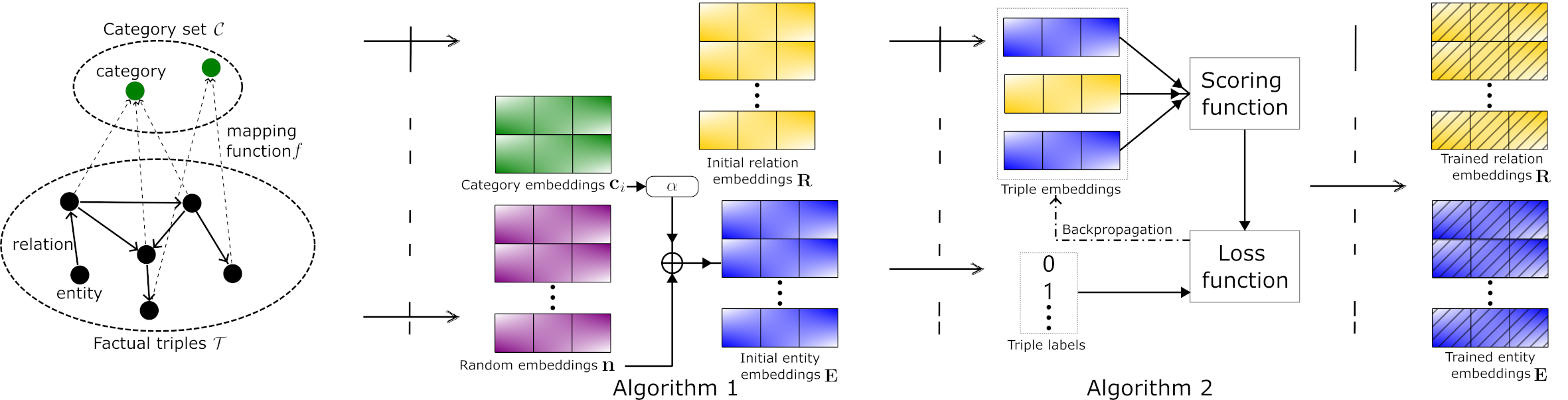
Category-centric KGE initialization
1. Introduction
Knowledge graph embedding (KGE) 1,2,3 has emerged as a core technique in machine learning for representing structured symbolic knowledge in a continuous embedding space. This technique maps entities and relations in knowledge graph triples (represented as (head entity, relation, tail entity)) into low-dimensional dense embeddings. The interactions among these embeddings serve to knowledge graph completion (KGC) 4 that estimates the plausibility of unseen or missing triples, effectively addressing the inherent incompleteness of real-world knowledge graphs. In addition, KGE has proven indispensable in a wide array of downstream tasks, including recommendation systems 5,6,7,8, biomedical systems 9,10, search engine 11, financial industry 12,13, and multimodal data 14,15.
To further enhance the utility of KGE, extensive research has focused on improving its effectiveness, such as by developing a more sophisticated scoring function to capture various relation patterns 16,17,4,18,19, or designing a more rational negative sampling mechanism to improve the quality of embeddings 18,20,19,21. Although these attempts have enhanced the expressiveness of KGE models, efficiency remains a bottleneck as the knowledge graphs continue to scale up. For example, WikiKG90Mv2 dataset has 91,230,610 entities, 1,387 relations, and 601,062,811 triples in total 22. At such a scale, even polynomial-complexity KGE models need over 10 billion parameters to learn effectively.(1) The staggering cost of training such a model limits the utility of KGE. In an effort to reduce training cost, some researchers have reduced the number of parameters by integrating sub-word embedding 23 into KGE models 24,25,26.
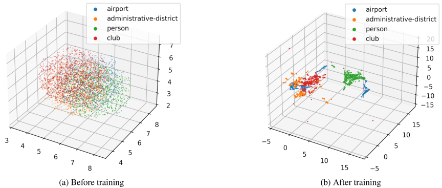
Fig. 1. Visualization of category-specific entity distributions in a KGE model.
However, one aspect that remains under-explored is the initialization strategy for KGE, which also plays a critical role in reducing the training cost 27. Although the importance of initialization as another approach in KGE has been pointed out 28 and some studies 28,29 have shown that appropriate initialization can improve the final performance of KGE models, it has not been the main topic of studies in the KGE domain. Given that the training cost is a barrier to applying KGE to large-scale knowledge graphs, we decided to focus on initialization from the perspective of reducing the training cost.
Most KGE methods adopt a simple random initialization. This approach generates initial embeddings from a random distribution (e.g., normal distribution or uniform distribution), which has the advantages of low cost and wide applicability. However, it comes with the risk of gradient explosion and gradient vanishing, which can severely impact the final performance of the model. For solving this problem, Xavier initialization 30 and orthogonal initialization 31 have been proposed. Xavier initialization stabilizes the variance during the training process by scaling the variance of the initial embeddings, thereby ensuring the stability of gradients. Orthogonal initialization introduces orthogonal matrices as initial matrices, whose rows can be regarded as initial embeddings for entities, to ensure that the norm of the error terms remains unchanged during backpropagation, thus also avoiding gradient explosion and vanishing.
Although such initialization reduces the computational cost, it also forfeits the ability to leverage prior knowledge, which is believed to hold potential for accelerating model training and enhancing model performance 20. To better utilize prior knowledge in knowledge graphs, methods that implement pre-training initialization have emerged 32,33,34,35,36. These methods obtain embeddings containing prior knowledge by means of pre-trained models and then use them as the initial embeddings for the next training. Such methods can be categorized into structural pre-training and textual pre-training on the basis of the types of information utilized.
Structural pre-training initializations 32,35,36 attempt to incorporate the graph-structured knowledge in the initial embeddings. Because of the complexity of modeling structural information, such methods are often intricate and come with a high computational cost.
Textual pre-training initialization extracts word embeddings corresponding to text labels from pre-trained language models (LMs) and uses them as initial embeddings. However, LMs lack specific training for dense knowledge, which reduces the performance of KGE models to some extent 34. A more pressing problem for such methods is their reliance on explicit text labels. In some scenarios, such as those involving confidential data where only entity and relation IDs are provided, these methods become inapplicable.
To address the above problems, we propose category-centric initialization (CCI), which incorporates category information into the initialization. Category information, as the most easily obtainable prior knowledge, is often included in knowledge graphs as auxiliary information.
KGE models, even when trained on data without explicit categories, tend to encompass category information in their distribution at convergence 37. This can be observed in Fig. 1, which shows the distribution of entity embeddings in a KGE model trained without utilizing explicit category information. The embeddings are color-coded according to category. We can see here that entities of the same category form a cluster in the distribution after training. Therefore, incorporating category information in the initialization is expected to make the entity’s initial distribution closer to the distribution at convergence, thereby shortening the time required to form the distribution at convergence. This could contribute to reducing the model’s training time and even further improving the model’s final performance.
The proposed method combines the embedding of the entity’s corresponding category with a random embedding to serve as the entity’s initial embedding. We introduce a hyperparameter to control the balance between prior knowledge and randomness. The embeddings of explicit categories are generated through random initialization, which can effectively reduce the cost of introducing prior knowledge. Thus, CCI can introduce prior knowledge at a low cost without pre-training. Since it does not utilize a pre-trained model or rely on explicit textual labels, it can be adapted to any scenario where a KGE model is trained from scratch.
We also consider a scenario where categories are implicitly available. In such a case, classification algorithms (e.g., Weisfeiler–Leman (WL) algorithm 38) can be used to generate category information for CCI. Therefore, CCI can be adapted to any scenario with or without explicit categories.
The main contributions of this paper can be summarized as follows:
-
We propose CCI as a first attempt to incorporate category information into the initialization of KGE models, which makes it possible to incorporate prior knowledge without pre-training.
-
We conduct experimental comparisons of multiple random initializations across two datasets and four KGE models, from both vertical and horizontal perspectives, and show that CCI can effectively and robustly reduce the training costs of advanced KGE models on KGC.
-
We clarify the effect of the balance between prior knowledge and randomness on CCI.
-
We show that CCI can be applied in scenarios without explicit category information by utilizing category information generated through the WL algorithm.
-
Our experimental code for CCI is based on PyKEEN 39, a comprehensive KGE library. Thus, CCI can be easily integrated into many KGE models. Our code is open-sourced.(2)
2. Related Work
2.1. Knowledge Graph Embedding Approaches and Applications
KGE refers to the methods that project elements of knowledge graphs into a continuous embedding space. These methods have been extensively developed over the years as means of exploiting knowledge graphs.
KGE methods focus on how to model the structural knowledge contained in triples. One category of these methods is based on the distance hypothesis to measure the confidence of triples.
TransE 4 first demonstrated the effectiveness of the distance hypothesis. This method assumes that the tail entity in a factual triple is the head entity after being “translated” by the relation and computes the embedding distance between the head and tail entities as the confidence of this triple. However, such a simple translation cannot handle relation patterns of symmetry. To solve this problem, RotatE 19 expands the embedding space to the whole complex space and learns the representations of entities and relations by considering relations as rotation operations between entities. Due to the properties of complex space, this method can model relation patterns of symmetry/antisymmetry, inversion, and composition.
Another category of KGE methods, known as bilinear models, is based on tensor decomposition. DistMult 16 utilizes diagonal matrices to learn multi-relational data. However, this method is unable to model symmetric relation patterns. ComplEx 17 extends DistMult into the complex embedding space by introducing complex conjugation to model asymmetric relations. ComplEx-N3 40 replaces the standard regularization in ComplEx by introducing tensor nuclear 3-norm regularization 41, in order to improve the performance of ComplEx on the KGC task.
KGE has been applied to knowledge graph-centric tasks such as KGC 4 (a.k.a., link prediction), which predicts missing links by ranking candidate triples; triple classification 42, which determines the validity of given triples by threshold; entity typing 37,43,44,45,46,47, which assigns missing types (categories) to entities; and relation extraction 48,18, which uses learned embeddings to identify and extract semantic relationships between entities from unstructured text.
Beyond these canonical tasks, KGE has also been used for practical purposes. In particular, it has been used in recommendation systems to enhance the representations of users and items 5,6,7, and its scope has been extended to include specialized tasks such as scholarly community recommendation 8 and educational content recommendation 49. In the biological domain, KGE has proven well-suited for representing biological systems 9 and has been applied to tasks such as drug interactions 50,51 and the prediction of drug polypharmacy side effects 10. As well, its application to search engines can enrich query understanding and document ranking through structured knowledge integration 11. In the financial industry, KGE captures complex knowledge to enhance tasks such as loan default risk prediction 12, stock price movement prediction 13 and financial report quality detection 52. In multimodal settings, semantic knowledge modeled by KGE has been integrated into video features 14 and music features 15.
Because of the effectiveness and efficiency of KGE in modeling multi-relational data and integrating structured information, we believe it also holds promise for such applications as federated recommendation 53, Quality-of-Service prediction 54, autoscaling for microservice-based applications 55, and knowledge-enhanced retrieval-augmented generation 56.
2.2. Initialization for KGE
The initialization challenge with KGE lies in how to set the initial values of learnable parameters, and it was first pointed out by researchers studying neural networks 57. Appropriate initialization can help models converge faster and even improve their final performance 27. Since KGE models, which utilize embeddings to represent entities and relations, can be regarded as special cases of single-layer neural networks, initialization also has a profound impact on them.
The initialization for KGE focuses on how to initialize the embeddings of entities and relations to help the model reach the distribution at convergence faster. In this section, we categorize the initialization for KGE into two types based on whether to use pre-trained embeddings: random initialization and pre-training initialization.
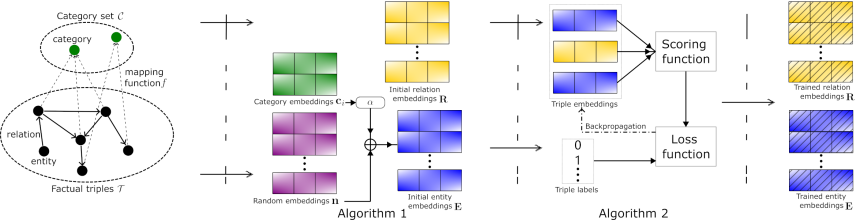
Fig. 2. Diagram of proposed method for KGE.
2.2.1. Random Initialization
A general choice for KGE models is simple random initialization. The most common methods utilize a standard normal distribution \(\mathcal{N}(0, 1)\) or uniform distribution \(\mathcal{U}(0, 1)\) to initialize the model. However, for KGE models, if the magnitude of the initial embeddings is not restricted, it is necessary to carefully design a learning rate adjustment strategy: if embedding norms are too large, gradients can become excessively large, causing the learning rate to overshoot the global optimum. To achieve the global optimum, the learning rate needs to be reduced at the appropriate time. However, deciding when and by how much to reduce the learning rate is a difficult problem. Therefore, a more common practice is to incorporate L2-normalization into the random initialization to limit the magnitude of the initial embeddings to 1. In this way, the model can achieve good results even without using a learning rate adjustment strategy.
However, simple random initialization does not consider the effect of the variance of the embeddings, which can lead to gradient vanishing or gradient explosion problems. Therefore, Glorot and Bengio 30 mathematically derived a method to scale the variance of embeddings, ensuring the consistency in the variance of both inputs and outputs. In this way, they improved the stability of the training and accelerated the convergence of the model. Specifically, for the standard normal distribution, Xavier initialization scales the standard deviation to \(\sqrt{2/\mathit{dim}}\), where \(\mathit{dim}\) represents the dimensionality of the embeddings. For the uniform distribution, they changed the bound and got the distribution \(\mathcal{U}(-\sqrt{6/\mathit{dim}}, \sqrt{6/\mathit{dim}})\).
In addition to keeping the variance consistent, another approach is to keep the gradient norms consistent. Saxe et al. 31 proposed using orthogonal matrices as the initial matrices, whose rows can be seen as initial embeddings for entities. Specifically, their method randomly initializes a matrix from the standard normal distribution and then obtains an orthogonal matrix through QR decomposition. The use of orthogonal matrices ensures that the error terms have norm-preserving properties, thereby improving the stability of the training.
2.2.2. Pre-training initialization
Pre-training initialization refers to an initialization that uses the embeddings obtained from a pre-trained model as the initial values for KGE models. KG-BERT 34 is one of the earliest models to use pre-trained representations directly. Instead of extracting pre-trained embeddings from BERT 58 for entities and relations, it directly fine-tunes the BERT model on the KGC task. However, this method does not perform as well as other KGE models, such as RotatE and ComplEx, on the KGC task.
The performance of KG-BERT on KGC is limited by the fact that the pre-trained language model (BERT) was not trained on knowledge-intensive data. Therefore, Kocijan and Lukasiewicz 33 proposed joint use of an RNN-based encoder and a KGE model for training on a large open knowledge graph dataset. They used embeddings obtained from the pre-trained model to initialize a KGE model and then fine-tune it on another small dataset.
However, similarly to KG-BERT, this method also requires that entities have explicit textual labels, and it cannot be applied to datasets without such information. One approach to avoiding this problem is to use structural information. Chung and Whang 32 clustered entities on the basis of structural similarity to generate a more compact meta-graph and used it to pre-train a KGE model. The pre-trained embeddings of a cluster are used as the initial embeddings of all entities belonging to it. HARP 35 adopted edge and star collapsing to create a hierarchical sequence of subgraphs, on which embeddings are pre-trained. These embeddings are then refined and used as the initial embeddings of entities. GPA 36 utilized another graph compression algorithm 59 to generate subgraphs while minimizing the information loss. The embeddings learned on these subgraphs are used as the initial entity embeddings. Although these methods improved the performance of models on link prediction tasks, they require high computational costs especially for large-scale knowledge graphs.
3. Category-Centric Initialization
In light of the above background, we propose CCI, which incorporates prior knowledge in the form of category information into the initialization at a low computational cost.
Figure 2 illustrates how CCI is incorporated in KGE. Specifically, it begins by acquiring embeddings for the categories, which are then summed with a random embedding to serve as an initial embedding of entities. A hyperparameter \(\alpha\) (\(\in [0,1]\)) is introduced to balance the apriority and randomness in the initial distribution of entity embeddings. The embeddings of entities and relations obtained by CCI are then used to compute scores for triples. Then, on the basis of these scores and the corresponding labels (1 for existing triples and 0 for unseen ones), the backpropagation algorithm 60 is used to update the embeddings, as is usually done in the training phase of conventional KGE models. The details of CCI are described in Algorithm 1, where the mapping function \(f: \mathcal{E} \rightarrow \mathcal{C}\) represents the correspondence between entities and categories, and \(c_n\) is the number of categories. In CCI, the embeddings of categories \(\boldsymbol{C} \in \mathbb{R}^{c_n \times d}\) are initialized using standard normal initialization. On line 2, \(\boldsymbol{c_i} \in \boldsymbol{C}\) is the embedding of the category to which entity \(e_i\) belongs. When \(e_i\) belongs to multiple categories, \(\boldsymbol{c_i}\) will be the average of their embeddings. On line 3, random initialization is used to generate an embedding \(\boldsymbol{n}\) to enhance the distinguishability of entities belonging to the same category. L2 normalization (\(P(\boldsymbol{x})\)) is used to adjust the norm of the initial embedding, thereby reducing the sensitivity of the model’s final performance to the learning rate. When the random initialization uses L2 normalization and \(\alpha\) is small enough, further normalization is unnecessary and \(P(\boldsymbol{x})\) should be an identity function.
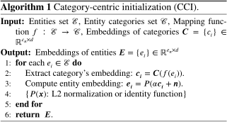
Unlike pre-training initialization, CCI does not rely solely on prior knowledge for initialization; it also uses randomness. We expect that an initial distribution that simultaneously incorporates randomness and prior knowledge will get closer to the final ideal distribution, which arranges the entities of the same category close together. One of the concerns when using category information is that it inherently has flaws, such as incompleteness. If this is not properly addressed, it will degrade the final performance of the model. Introducing randomness is also an effective countermeasure against this issue.
In the following, Section 3.1 describes the base KGE models that can be integrated with CCI, explains why these models were chosen, and shows their score functions. Section 3.2 describes how to optimize and train these KGE models initialized by CCI.
3.1. Base Models
Table 1. Models, scoring functions, and parameters used in experiments. normal represents the standard normal distribution; xavier_uniform represents the Xavier uniform distribution; *_norm denotes the additional use of L2 normalization.
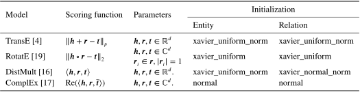
To evaluate the effectiveness of the proposed method across KGE models of various complexity and types, i.e., from distance-based to bilinear, we examined two simpler models, TransE 4 and DistMult 16, and two advanced models, RotatE 19 and ComplEx 17.
Table 1 summarizes the scoring functions, the model parameters and their ranges, and their default initialization. In this table, \(\boldsymbol{h}\), \(\boldsymbol{r}\), and \(\boldsymbol{t}\) denote the embedding of the head entity, relation, and tail entity, respectively. \(\mathbb{R}^d\) and \(\mathbb{C}^d\) denote a \(d\)-dimensional real number space and complex number space, respectively. \(\lVert * \rVert_p\) denotes the p-norm. \(\langle \cdot \rangle\) denotes the generalized dot product. \(\text{Re}(\boldsymbol{x})\) and \(\bar{\boldsymbol{x}}\), respectively, denote the real part and conjugate of a complex embedding \(\boldsymbol{x}\).
TransE and DistMult share the same initialization and use the real number space for embeddings. In contrast, RotatE and ComplEx are embedded in the complex number space and thus have more expressive power.
3.2. Optimization and Training
After initialization, KGE models require further optimization on the loss function. Ali et al. 29 have shown that different types of KGE models should use different loss functions for optimal performance.
For the distance-based models (TransE and RotatE), we chose the self-adversarial negative sampling loss 19. The core idea of this loss function is to generate negative weights based on the scores of negative samples, thereby helping the model to focus on high-quality negative samples. It is calculated as
For the bilinear models (DistMult and ComplEx), we chose the cross-entropy loss, which is widely utilized in machine learning. It can be represented as
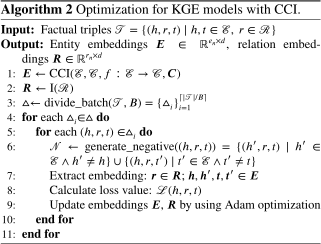
Algorithm 2 illustrates the detailed training process of KGE models with CCI. In this algorithm, entity embeddings \(\boldsymbol{E} \in \mathbb{R}^{e_{n} \times d}\) are initialized using CCI, where \(e_{n} = |\mathcal{E}|\) is the number of entities. Relation embeddings \(\boldsymbol{R} \in \mathbb{R}^{r_{n} \times d}\) are initialized using the default initialization \(I(\mathcal{R})\) in Algorithm 2, where \(\mathcal{R}\) is the relations set and \(r_{n} = |\mathcal{R}|\) is the number of relations. On the basis of the stochastic local closed world assumption 29, all unseen triples are labeled 0, a batch of factual triples \(\vartriangle_i\) is randomly sampled from the factual triples \(\mathcal{T}\) (line 3), and a finite number of negative samples \(\mathcal{N}\) are constructed by randomly replacing the head or tail entity of the factual triple (line 6). On line 3, \(\lceil * \rceil\) is the ceiling function, and \(B\) is the batch size. A KGE model is used to calculate the loss values for these triples (line 8). The loss value is minimized by using the Adam optimizer 61 to update the embeddings of the entities and relations (line 9).
4. Experiments
4.1. Datasets
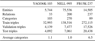
Three datasets with explicit category information were utilized: YAGO6K-103, NELL-995, and FB15K237. YAGO6K-103 is a smaller dataset, with only 30K training triples; it was derived by filtering out entities without explicit categories from YAGO26K-906 62. NELL-995, featuring over 138K training triples, was obtained by Xiong et al. 63 by filtering out valueless relations from the 995th iteration of the NELL system 64. FB15K237 65 is a refined version of the FB15K 4 that addresses the test set leakage issue. In our experiments, we chose to use the cleaned category information for FB15K237 provided by 21. It is worth noting that the average number of categories per entity in FB15K237 is significantly larger than in the other two datasets. Table 2 lists detailed information about these three datasets. All datasets contain explicit category information as triples, e.g., (Chelsea_F.C., isa, club), (Rekha, isa, person), (China, isa, country) in YAGO6K-103, (nicholas_nickleby, isa, movie), (\((-10.29444, -76.89111)\), isa, coordinate), (siula_grande, isa, mountain) in NELL-995 and (/m/0g9zljd, isa, award), (/m/04glr5h, isa, book), (/m/016cff, isa, sports) in FB15K237.
Table 2. Dataset statistics. Average categories indicates the average number of categories assigned to each entity.
4.2. Experimental Settings
The experiments using the NELL-995 and FB15K237 datasets were conducted on an NVIDIA GeForce RTX 3090, and those using the YAGO6K-103 dataset were conducted on an NVIDIA GeForce RTX 3080 Ti. For a fair comparison of initialization performance, we fixed the hyperparameters across all base models as in 36. Specifically, we set the batch size to 512, the maximum epochs to 200, the embedding dimensionality to 768, and 64 negative samples for each positive triple. The learning rate for each model was chosen from \(\{0.001, 0.0001\}\). The experimental code was based on PyKEEN 39, a comprehensive code library that integrates multiple KGE models; note that this makes the proposed method easily applicable to many models. The experimental code is publicly available.(3)
To avoid unnecessary computation, we adopt an early stopping strategy during training. Early stopping has been validated since the early neural network literature 66 as an effective way to curb overfitting and reduce training costs, and it remains a widely used practice in modern deep learning 67,68,69. It is also commonly applied in KGE field 4,29. Specifically, the model is evaluated every \(s\) epochs, and if the improvement in the metric is less than \(\delta\) for \(m\) consecutive times, training is terminated, and the best model obtained so far is evaluated with a test set. In the experiments, \(s=5\), \(\delta = 0.0001\), and \(m=6\) were common settings, except for the models that converged quickly; in those cases, \(s\) was set to 1.
4.3. Experimental Task and Evaluation Protocol
KGC is a commonly used task to evaluate the performance of KGE models. This task requires the model to infer the answer entity to a query (head entity, relation, ?) or (?, relation, tail entity) based on known factual triples. Generally, a model computes a score for each candidate entity and selects the entity with the highest score as the answer entity.
The most commonly utilized metric to evaluate KGE models on the KGC task is the mean reciprocal rank (MRR), which is defined as
In the experiments, MRR was used not only to measure the model’s final performance on the test set but also in the early stopping strategy to decide whether to terminate training.
In addition, we devised two metrics for horizontal and vertical comparisons: \(\mathit{Epoch}\) and \(\mathrm{Epoch}_{l}\). \(\mathit{Epoch}\) measures the convergence speed of a model and is defined as the epoch number at which a model’s MRR value first exceeds a specified accuracy requirement. This metric provides a basis for horizontal comparison, as it evaluates different initializations on the same accuracy threshold for each model. \(\mathrm{Epoch}_{l}\) is defined as the number of epochs at which training stops when the early stopping \(\delta\) is set to a value of \(l\). This metric reveals the performance of each initialization under different early stopping settings. To cover more scenarios, we set \(l = \{0.01, 0.001, 0.0001\}\).
4.4. Experimental Results
4.4.1. Experiments with Explicit Categories
To evaluate the effectiveness of CCI, we first conducted an experiment on scenarios with explicit category information. Three initializations without using pre-trained models were selected as baselines: xavier, simple, and orthogonal. Among these, xavier and simple had four variations: normal distribution and uniform distribution, and normal distribution and uniform distribution with L2 normalization—resulting in a total of nine baseline variants. These baselines were used not only for comparison with CCI but also for generating random embeddings \(\boldsymbol{C}\) and \(\boldsymbol{n}\) in Algorithm 1. On the basis of the best-performing baseline initialization, four variations of CCI with different proportions of the category embedding were tested, where \(\alpha \in \{0.002, 0.004, 0.01, 0.02\}\). While our main experiments focus on these random initializations due to their scalability and broad applicability, we also report additional comparisons against a structural pre-training-based initializer and provide the corresponding analysis in Appendix B.
For different models and datasets, all hyperparameter settings were held constant except for the learning rate and loss function. Moreover, for each individual model, the same learning rate and loss function were used across all initialization methods.
Table 3. Vertical comparison results on YAGO6K-103.
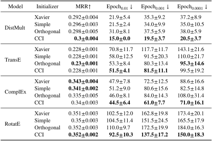
Table 4. Vertical comparison results on NELL-995.
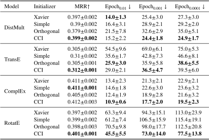
Table 5. Vertical comparison results on FB15K237.
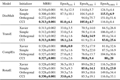
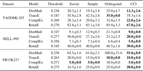
Table 6. Epochs required to exceed model-specific MRR thresholds across datasets. Each setting was repeated over ten times under different random seeds and shown as \((\text{mean} \pm \text{std})\). A lower value is better.
In the vertical comparison, different \(\mathrm{Epoch}_l\)s, i.e., Epochs with different values of \(l\), were obtained from the same experimental result. Tables 3–5 present the results. In these tables, MRR represents the final results on the test set with \(\delta = 0.0001\). \(\mathrm{Epoch}_{l}\) shows the results for when \(\delta = l\) in the early stopping strategy. Each setting was repeated more than ten times under different random seeds, indicated as \((\text{mean} \pm \text{std})\). ↑ (↓) means a higher (lower) value is better. To determine the best performance, we compared the results as follows: for metrics where higher is better (↑), \((\text{mean} - \text{std})\) is compared; for metrics where lower is better (↓), \((\text{mean} + \text{std})\) is compared. The best results are highlighted in bold.
For initializations that have multiple variations, we first filtered out those variations whose results are below 95% of the best validation result. This filtering excludes cases that significantly degrade the model’s performance. Then, from those, the results with the smallest sum of the three \(\mathrm{Epoch}_l\)s are selected as the best result for this initialization and displayed in tables.
On the YAGO6K-103 dataset, for DistMult and RotatE, CCI significantly reduced the epochs under various settings of \(\delta\) while maintaining the same level of MRR. For ComplEx, CCI reduced the epochs when \(\delta\) was set to 0.001 and 0.0001. However, for TransE, CCI exhibited no improvement when compared with orthogonal initialization. On the NELL-995 dataset, for RotatE, CCI greatly reduced the epochs. CCI also brought improvements to ComplEx, although it converged quickly regardless of the initializer. For TransE, CCI significantly improved the model’s final performance compared with Orthogonal, but was slower. Although the final performances of CCI and Simple were similar, CCI reduced the number of epochs. For DistMult, CCI reduced the number of epochs when \(\delta\) was set to 0.001 and 0.0001. On the FB15K237 dataset, DistMult initialized with the orthogonal method exhibited highly unstable results, and even failed to converge when \(\delta\) was set to 0.01. In contrast, CCI not only achieved the best overall performance but also yielded better results for both \(\delta = 0.01\) and \(\delta = 0.001\). Although Simple achieved the best result when \(\delta\) was set to \(0.0001\), its MRR was obviously worse than CCI’s. For ComplEx, CCI had more stable results when \(\delta\) was set to \(0.001\) and \(0.0001\), without sacrificing performance. For TransE and RotatE, CCI achieved the best MRR, although the improvement in convergence speed is limited.
By comparing the results on the YAGO6K-103 and NELL-995 datasets, we found that for the advanced models based on complex number space, such as RotatE and ComplEx, CCI effectively reduced the number of epochs in various convergence settings regardless of the dataset. On the other hand, regarding the simpler models, DistMult and TransE, it had a noticeable difference in performance between datasets: CCI performed better for DistMult on the smaller YAGO dataset. In contrast, for TransE, it performed better on the larger NELL-995 dataset. However, the effect of CCI was relatively small on the FB15K237 dataset. We attribute this to the high average number of categories per entity in this dataset. Since CCI initializes each entity based on the averaged representation of its associated categories, such a strategy may introduce ambiguity when an entity is linked to too many categories. Compared with the other two datasets, this ambiguity weakens the clustering effect of the initialized embeddings in FB15K237, thereby diminishing the advantage of CCI in reducing the training cost.
The results on YAGO6K-103 and NELL-995 indicate that the CCI initialization performs inconsistently on simple KGE models like TransE and DistMult, being easily affected by the statistics of the dataset. However, for more advanced and complex models, CCI has the ability to reduce the training cost of the model without impacting its performance, regardless of the dataset. At the same time, the results on FB15K237 reveal a limitation in handling entities associated with multiple categories.
In Tables 3–5, we can see that the standard deviation (std) of the \(\textrm{Epoch}_{l}\) was large relative to the mean regardless of initializers. Despite each experimental method being repeated more than ten times, it did not completely eliminate the influence of randomness on the results. Therefore, in the horizontal comparison, the accuracy requirement should be set below optimal performance to ensure that models can always meet it. In the experiments, the accuracy requirement (MRR threshold) was set to 90% of the optimal validation result for each model.
Table 6 presents the results of the horizontal comparison, and the corresponding curves are provided in Appendix A. Compared with the results of the vertical comparison, the std in the horizontal comparison results was small relative to the mean. Therefore, the performance of the initialization demonstrated in the horizontal comparison was more deterministic.
For the YAGO6K-103 dataset, as shown in Table 6, the proposed method achieved the lowest mean and std of Epoch on both the ComplEx and RotatE models, reflecting its effectiveness. For DistMult, although the std of CCI was higher than the lowest one (Xavier), its mean was significantly lower than those of the baselines. On TransE, however, CCI was slightly worse than orthogonal. For the NELL-995 dataset, CCI achieved the lowest mean and std across all models, although the improvement with the DistMult model was not considered significant. For the FB15K237 dataset, CCI achieved the lowest mean and standard deviation on both RotatE and DistMult. Although the baseline and CCI performed equally well on TransE and ComplEx, CCI exhibited a standard deviation of 0 across all models. Furthermore, CCI consistently demonstrated more stable performance across all datasets.
From the horizontal experimental results on all datasets, we can draw the same conclusion as in the vertical comparison: CCI can effectively and robustly reduce the time required to transit from the initial distribution to the distribution at convergence in advanced KGE models on the YAGO6K-103 and NELL-995 datasets. This means it can effectively lower the training costs for advanced KGE models in scenarios where entities are associated with fewer categories. On the FB15K237 dataset, although CCI achieved the best result, the difference from the baselines was relatively small. This result shows the limitation of CCI in dealing with scenarios where entities tend to have multiple categories.
For completeness, we also provide the curves of how MRR changes during training under different initialization methods, together with the corresponding analysis, in Appendix A.
4.4.2. Ablation Results
Table 7. Vertical ablation results on NELL-995.
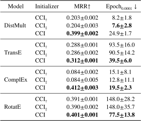
We conducted ablation experiments on NELL-995 to evaluate the impact of the balancing parameter and the random embedding used in CCI under vertical setting. All other hyperparameters were kept fixed. Here, CCI\(_{†}\) denotes the variant where \(\alpha = 1\), and CCI\(_{‡}\) further removes the random embedding \(\boldsymbol{n}\) under the same condition, effectively using the pure category embedding as the initial entity embedding.
Table 7 shows the ablation results of the vertical comparison, where MRR refers to the performance on the test set with \(\delta=0.0001\), and \(\textrm{Epoch}_{0.0001}\) represents the number of epochs required to reach this result. The ablated variants had a substantial performance degradation relative to full CCI on DistMult and ComplEx, with their final MRRs dropping to 50% and 20%. In contrast, for TransE and RotatE, the final MRRs of the ablated models were 92% and 97% of full CCI’s MRR. Both ablations also significantly underperformed the full CCI on \(\textrm{Epoch}_{0.0001}\). These results highlight the importance of both the balancing parameter and the injected randomness when initializing entities based on category information.
Moreover, we found that the ablated variants exhibited similar performance across all models, which prompted us to conduct a further investigation on the effect of the balancing parameter \(\alpha\).
4.4.3. Impact of \(\alpha\)
The parameter \(\alpha\) in Algorithm 1 determines the proportion of category embeddings in the initial embeddings of entities. This value directly affects the clustering degree of entities in the embedding space, which in turn affects the performance improvement brought by CCI.
To analyze the impact of \(\alpha\), we used the Caliński–Harabasz (CH) score (also known as the variance ratio criterion) 70 to quantify the clustering degree induced by CCI. The definition is
For CCI, \(\boldsymbol{p}_i\) is defined as \(\boldsymbol{e}_i\) on line 3 of Algorithm 1:
Assuming \(P(\cdot)\) is the identity function and each entity belongs to exactly one category, Eq. 5 can be rewritten as
Assuming both \(\boldsymbol{c}\) and \(\boldsymbol{n}\) consist of independent and identically distributed (i.i.d.) components, and are independent of each other, the expectation of Eq. 8 is
To understand how category embeddings affect the clustering score, we focus on the expectation of \(A\).
As \(e_n\) and \(c_n\) are constants, the expected CH index increases quadratically with \(\alpha\), given a fixed \(d\) and initialization for the random embedding \(\boldsymbol{n}\).
Table 8 shows CH scores for different \(\alpha\) when L2 normalization is used as \(P(\cdot)\). As L2 normalization only preserves the direction of each embedding, the cluster centers are no longer \(\alpha\boldsymbol{c}_i\), and Eq. 13 does not hold strictly. Even so, the CH score is approximately proportional to \(\alpha^2\) when \(\alpha\) is sufficiently large (e.g., from 0.01 to 0.04). However, this relationship disappears when \(\alpha\) is small. We think that L2 normalization breaks down the independence assumption behind Eq. 13.
Table 8. CH scores under different values of \(\alpha\) when \(P(\cdot)\) is L2 normalization.

Nevertheless, \(\alpha\) serves as a control parameter for adjusting the degree of initial clustering. Since the optimal degree of clustering is unclear across different datasets and KGE models, \(\alpha\) is treated as a hyperparameter and is typically selected through trial-and-error.
To investigate its effect, we examined how different values of \(\alpha\) affect the performance of the proposed method. In the following experiments on scenarios with explicit category information, \(\alpha\) was set to \(\{0.002, 0.004, 0.01, 0.02\}\).
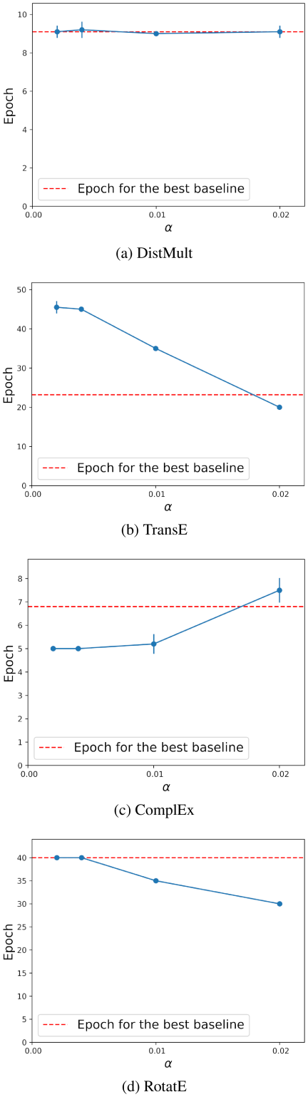
Fig. 3. Ablation on NELL-995: CCI with different \(\alpha\) across base models. Dots indicate mean epochs; vertical bars denote standard deviation.
Figure 3 shows the number of epochs needed to reach the accuracy requirement on the NELL-995 dataset. We can see here that for the distance hypothesis-based KGE models, TransE and RotatE, Epoch decreased as \(\alpha\) increased, which implies that Epoch may further decrease with larger \(\alpha\). In contrast, for ComplEx, an optimal \(\alpha\) seemed to exist within the range tested. For DistMult, Epoch was insensitive to \(\alpha\). A similar tendency was observed on the YAGO6K-103 and FB15K237 datasets, except for DistMult, which achieved the smallest Epoch when \(\alpha\) was set to 0.01 on YAGO6K-103 and 0.02 on FB15K237.
To investigate whether a larger \(\alpha\) could further reduce Epoch for TransE and RotatE, we conducted an additional experiment with a larger range of \(\alpha\). Fig. 4 shows the results of TransE on the NELL-995 dataset. Here, we can see that Epoch was smallest when \(\alpha\) was around 0.02. A similar tendency was observed for RotatE.
The experimental results demonstrate that Epoch was affected differently by \(\alpha\), which controls the degree of entity clustering, for different types of KGE models. For the distance hypothesis-based KGE models, Epoch was smallest when \(\alpha\) was around 0.02. In contrast, for the bilinear models with CCI Epoch was smallest when \(\alpha\) was set to 0.02, 0.01, or 0.004. The difference in Epoch’s behavior arises from the different scoring functions and loss functions used by these models, but an investigation on this topic will have to be left to future work.
4.4.4. Experiments Without Explicit Categories
To test whether the proposed CCI can be used in scenarios without explicit category information, we replaced the explicit category information of the NELL-995 dataset with categories generated by the WL algorithm 38. This algorithm classifies nodes in a graph by iteratively aggregating the structural features of the nodes and their adjacent nodes. By applying it to the NELL-995 dataset, 75,536 entities were divided into 15,728 categories. For this experiment, we used the advanced KGE model, RotatE, as the base model.
The experimental results are shown in Table 9. Here, Base represents the results of the random initialization Xavier, which were also used to initialize the category embeddings and random embeddings for CCI and CCI+WL. CCI represents the results using explicit categories. CCI+WL represents the results obtained using categories generated by the WL algorithm.
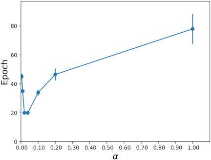
Fig. 4. Horizontal experimental results on NELL-995 for CCI with different \(\alpha\) on TransE. The dot represents Epoch’s mean, and the vertical line through the dot represents Epoch’s std.
Table 9. Vertical comparison results regarding category information on NELL-995.
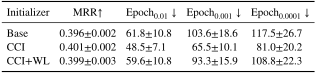
Compared with Base, \(\mathit{CCI} + \mathit{WL}\) reduced all \(\textrm{Epoch}_{l}\) values while achieving a higher MRR. This means that CCI can utilize category information generated by WL, thus demonstrating its applicability to scenarios without explicit category information.
It is also observed that CCI significantly reduced the epochs while maintaining the best performance. The only difference between CCI and CCI+WL is the category information. These results indicate that the quality of category information affects the performance of CCI, which underscores the rationale behind incorporating category information into the initialization process. In other words, it is a limitation of CCI: as generating reliable category information itself can be a challenging task, the most suitable application scenario for CCI remains datasets with explicit category information.
For datasets lacking such ground-truth category information, CCI may serve as a tool to evaluate the effectiveness of unsupervised graph clustering algorithms: the performance of CCI could be used as an indirect indicator of the quality of category information.
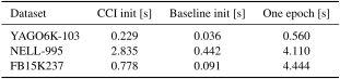
Table 10. Wall-clock time of initialization and training for RotatE. We report the absolute time [s] of CCI initialization, a standard baseline initializer, and one training epoch under the same training setting and hardware environment. The epoch time is independent of the initializer and is thus reported once per dataset.
4.4.5. Efficiency Analysis
We analyze both the asymptotic complexity and the practical wall-clock overhead of CCI. The time and space complexity of standard methods such as Xavier, simple, and orthogonal are all \(\mathcal{O}(e_n \times d + r_n \times d)\), where \(e_n\) and \(r_n\) denote the number of entities and relations, and \(d\) is the embedding dimension. In contrast, CCI incorporates category-level information during initialization, resulting in time complexity \(\mathcal{O}(e_n \times \bar{k} \times d + r_n \times d + c_n \times d)\) and space complexity \(\mathcal{O}(e_n \times d + r_n \times d + c_n \times d + \bar{k} \times d)\), where \(c_n\) is the number of categories and \(\bar{k}\) is the average number of categories per entity. Given that \(e_n \gg r_n\) and \(e_n \gg c_n \gg \bar{k}\) in all datasets, the complexities can be approximated as \(\mathcal{O}(e_n \times d)\) for the baselines and \(\mathcal{O}(e_n \times \bar{k} \times d)\) for CCI.
In practice, \(\bar{k}\) is small—approximately 1 for YAGO and NELL, and around 7 for FB15K237. Moreover, the time complexity for training a single epoch of a KGE model is approximately \(\mathcal{O}(|\mathcal{T}| \times d)\), where \(|\mathcal{T}|\) is the number of training triples. Even in the largest case (FB15K237), where \(|\mathcal{T}| = \textrm{272,115}\) and \(e_n \times \bar{k} \approx \textrm{101,535}\), we still have \(|\mathcal{T}| > e_n \times \bar{k}\). Therefore, the time cost of CCI is significantly smaller than that of a single training epoch of a model and is incurred only once at initialization. The additional cost introduced by CCI is thus negligible in comparison to the overall training time.
To further quantify the practical overhead, we additionally measure wall-clock time under the same environment(4) using RotatE as a representative model (Table 10). On YAGO6K-103, CCI takes 0.229 s while one epoch takes 0.560 s, corresponding to about \(0.229/0.560 \approx 0.41\) epoch; the baseline initializer corresponds to \(0.036/0.560 \approx 0.06\) epoch. On NELL-995, CCI corresponds to \(2.835/4.110 \approx 0.69\) epoch (baseline: \(0.442/4.110 \approx 0.11\) epoch). On FB15K237, CCI corresponds to \(0.778/4.444 \approx 0.18\) epoch (baseline: \(0.091/4.444 \approx 0.02\) epoch). Therefore, although CCI is slower than conventional random initializers due to incorporating category information, its overhead remains below one training epoch in all tested settings and is incurred only once at initialization.
5. Conclusion
In this paper, we addressed the initialization challenge that has long been overlooked in the KGE field and proposed an initialization called category-centric initialization (CCI). CCI is novel in that it introduces category information during initialization. Specifically, it uses a combination of embeddings related to entity categories and random embeddings for initialization, and it uses a hyperparameter \(\alpha\) to control the balance between prior knowledge and randomness. By using random initialization to generate category embeddings, prior knowledge can be incorporated into the initialization without pre-training, thus reducing the computational cost. This is ideal for scenarios where KGE models are trained from scratch.
Experimental results on the YAGO6K-103 and NELL-995 datasets demonstrated that CCI can effectively and stably reduce the training costs of advanced KGE models when entities are assigned to a few categories. For the scenarios involving entities with multiple categories, experimental results on the FB15K237 dataset demonstrated that CCI performs as well as or better than other initialization methods, even under ambiguous category information. The impact of \(\alpha\) on different KGE models was also clarified from both theoretical and empirical perspectives.
Furthermore, this paper also evaluated the performance of CCI using category information generated by the WL algorithm. The experimental results demonstrated its applicability to scenarios without explicit category information. At the same time, these results also suggested the importance of the quality of category information to the performance of CCI. This clearly narrows the scope of CCI’s applicability. Moreover, CCI is also not well-suited to handling multi-category scenarios. We envision that this flaw could potentially be addressed through heuristic ways, such as using category frequency as a weighting factor. We leave the exploration of this direction to future work.
Appendix A. Supplementary Plots for Horizontal Comparison
To complement the horizontal comparison results reported in the main text, we provide additional visualizations of the threshold-crossing behavior for different initialization methods. Specifically, we plot the validation MRR trajectories as a function of training epoch, truncated at the first epoch where the MRR exceeds a model-specific threshold. These figures illustrate, across multiple datasets and KGE models, how quickly each initialization strategy reaches the target performance level, thereby offering a more intuitive view of convergence efficiency. For clarity, we group the plots by dataset, and within each dataset we present one plot per model annotated with its corresponding threshold.
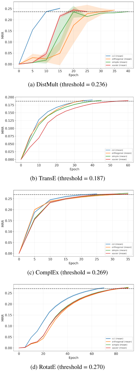
Fig. 5. YAGO6K-103: validation MRR curves as a function of epoch, truncated at the first epoch where MRR exceeds the model-specific threshold.
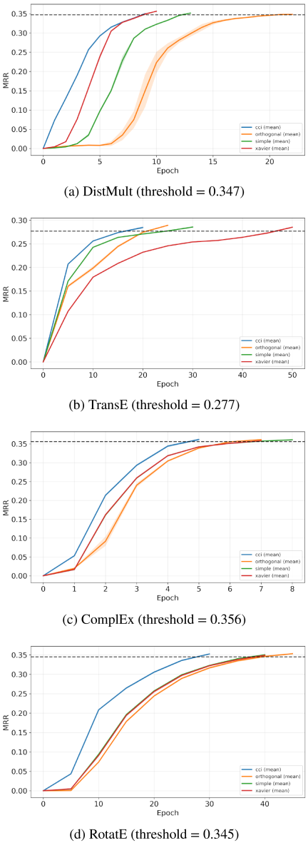
Fig. 6. NELL-995: validation MRR curves as a function of epoch, truncated at the first epoch where MRR exceeds the model-specific threshold.
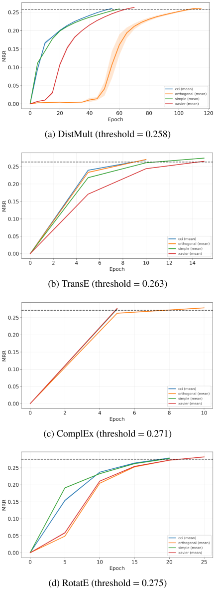
Fig. 7. FB15K237: validation MRR curves as a function of epoch, truncated at the first epoch where MRR exceeds the model-specific threshold.
Table 6 summarizes the horizontal comparison results in terms of the epochs required to exceed the model-specific MRR threshold (lower is better), while Figs. 5–7 provide a visual interpretation of when and how fast each initializer first surpasses the target threshold. Overall, the visualizations are consistent with the tabulated results: CCI typically reaches the target performance earlier than baselines.
As shown in Fig. 5, CCI exhibits a clear early-stage advantage on most models, where its mean MRR curve rises earlier and approaches the threshold more quickly. This observation aligns with Table 6, where CCI achieves the best mean epochs on DistMult (12.3 vs. 19.5–25.0), ComplEx (22.0 vs. 28.2–32.0), and RotatE (67.0 vs. 82.8–85.0). On TransE, however, Orthogonal slightly outperforms CCI (35.0 vs. 35.5), which is also reflected in Fig. 5(b) by the near-overlapping threshold-crossing points among all initializers. These results suggest that while CCI consistently accelerates convergence for more advanced models (e.g., ComplEx and RotatE), certain model–initializer combinations (e.g., TransE with Orthogonal) can remain competitive.
Figure 6 shows a consistent trend that CCI enters the rapid-improvement phase earlier and reaches the threshold ahead of baselines across all models. Correspondingly, Table 6 reports that CCI attains the lowest mean epochs for DistMult (9.0), TransE (20.0), ComplEx (5.0), and RotatE (30.0), yielding substantial reductions on TransE and RotatE compared with the best baselines (e.g., 20.0 vs. 23.2 and 30.0 vs. 40.0, respectively). For DistMult, the improvement is marginal (9.0 vs. 9.1), which is also visible in Fig. 6(a) as the curves converge rapidly and the threshold is reached within very few epochs.
As shown in Fig. 7, the differences among initialization methods become less pronounced on TransE and ComplEx, where the curves reach the threshold within very few epochs and largely overlap around the crossing point. This behavior is consistent with Table 6, in which several methods tie for the best mean epochs on TransE (10.0) and ComplEx (5.0). In contrast, on DistMult and RotatE, CCI still provides a noticeable acceleration (55.0 vs. 61.0–100.0 for DistMult; 20.0 vs. 24.5–25.0 for RotatE), matching the earlier rise of the CCI curve in Figs. 7(a) and (d). From a data perspective, the smaller gaps are also consistent with the limitation of CCI in settings where entities tend to be associated with multiple categories, thereby weakening the benefit of category-derived priors.
Overall, the horizontal visual results corroborate the main conclusion drawn from Table 6: CCI generally reduces the number of epochs required to reach a target performance level, with the most pronounced gains observed on YAGO6K-103 and NELL-995, especially for advanced KGE models. These results support the claim that incorporating category information at initialization can effectively shorten the warm-up phase and lower training costs, while the benefit becomes less distinguishable in scenarios where the threshold is reached almost immediately (e.g., FB15K237 on TransE/ComplEx) or where strong geometry-aligned initializers already perform competitively (e.g., YAGO6K-103 on TransE with Orthogonal).
Appendix B. Comparison with Structural Pre-Training Initialization
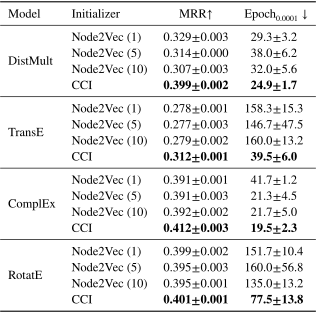
A practical concern for initialization strategies is whether the downstream gains are sufficient to justify the additional computational cost incurred at the initialization stage. To examine this time–performance trade-off, we compare CCI with Node2Vec 71, a general method for modeling structural information. Specifically, we use the Node2Vec-pretrained node representations to initialize KGE models and compare the resulting downstream performance and training efficiency against CCI on NELL-995 under the same training setting.
For the Node2Vec baseline, we follow the default configuration and vary only the number of training epochs to control the pre-training budget. Specifically, we set the return and in–out parameters to \(p=1.0\) and \(q=1.0\), the walk length to 100, and the context window size to 10. We then train Node2Vec for \(k\in\{1,5,10\}\) epochs (denoted as Node2Vec(\(k\)) in Table 11) and use the resulting node representations to initialize entity representations in the downstream KGE model.(5)
Table 11 shows that Node2Vec provides a reasonable initialization across models; however, CCI consistently achieves higher MRR and faster convergence (smaller \(\textrm{Epoch}_{0.0001}\)) in all cases. Notably, increasing the pre-training budget yields limited and sometimes negative effects. For example, for DistMult, Node2Vec(1) attains the best MRR among the three settings, while longer pre-training (5 or 10 epochs) degrades performance. This behavior indicates that additional structural pre-training does not necessarily translate into a better inductive bias for KGE, and may even introduce biases that are misaligned with the downstream scoring function and training objective. More broadly, we attribute the limited gains of Node2Vec to its original design target: it was developed for single-relation graphs, whereas knowledge graphs are inherently multi-relational. When Node2Vec is used as an initializer, collapsing multiple relation labels into an unlabeled graph discards relation-specific semantics, leading to a weaker and less targeted prior than CCI, which injects category-aware priors directly into entity representations.
Beyond accuracy and convergence, the wall-clock time of CCI initialization is 2.835 seconds. In contrast, Node2Vec with only one epoch already requires 172.710 seconds.(6) Therefore, even the lightest Node2Vec we tested costs approximately \(172.710/2.835 \approx 61\) times as much as CCI initialization. This overhead can become a bottleneck when frequent reruns are required for hyperparameter tuning or model selection. In comparison, CCI injects category priors with a lightweight procedure and achieves superior downstream performance and faster convergence, offering a more favorable time–performance trade-off.
Taken together, Table 11 and the wall-clock analysis indicate that structural pre-training (Node2Vec) initialization yields limited and unstable improvements, while incurring substantial additional computation. In contrast, CCI achieves consistently better inference performance and convergence efficiency with negligible extra initialization cost, making it a practical choice for KGE training.
Table 11. Vertical comparison between structural initialization (Node2Vec) and the proposed method (CCI) on NELL-995.
Acknowledgments
This work was partially supported by JST [Moonshot R&D][Grant Number JPMJMS2034] and JSPS KAKENHI Grant Numbers JP23K24953 and JP22K19836.
Footnotes
(1) https://ogb.stanford.edu/docs/lsc/leaderboards/#wikikg90mv2 [Accessed June 27, 2026]
(2) https://github.com/Scaredname/CCI [Accessed June 27, 2026]
(3) https://github.com/Scaredname/CCI [Accessed June 27, 2026]
(4) The measurements were conducted on a single machine with an Intel Core i7-12700K CPU (20 logical CPUs), 31 GiB RAM, and an NVIDIA GeForce RTX 3090 GPU.
(5) We use fastnode2vec, an optimized implementation of Node2Vec, to reduce the pre-training overhead: https://github.com/louisabraham/fastnode2vec [Accessed June 27, 2026]
(6) The reported Node2Vec time corresponds to Node2Vec(1) using fastnode2vec.
- [1] Q. Wang, Z. Mao, B. Wang, and L. Guo, “Knowledge graph embedding: A survey of approaches and applications,” IEEE Trans. Knowl. Data Eng., Vol.29, No.12, pp. 2724-2743, 2017. https://doi.org/10.1109/TKDE.2017.2754499
- [2] A. Rossi, D. Barbosa, D. Firmani, A. Matinata, and P. Merialdo, “Knowledge graph embedding for link prediction: A comparative analysis,” ACM Trans. Knowl. Discov. Data, Vol.15, No.2, Article No.14, 2021. https://doi.org/10.1145/3424672
- [3] X. Ge, Y. C. Wang, B. Wang, and C.-C. J. Kuo, “Knowledge graph embedding: An overview,” APSIPA Trans. Signal Inf. Process., Vol.13, No.1, 2024. https://doi.org/10.1561/116.00000065
- [4] A. Bordes, N. Usunier, A. Garcia-Durán, J. Weston, and O. Yakhnenko, “Translating embeddings for modeling multi-relational data,” Proc. 27th Int. Conf. Neural Inf. Process. Syst. (NIPS’13), Vol.2, pp. 2787-2795, 2013.
- [5] Y. Cao, X. Wang, X. He, Z. Hu, and T.-S. Chua, “Unifying knowledge graph learning and recommendation: Towards a better understanding of user preferences,” Proc. World Wide Web Conf. (WWW’19), pp. 151-161, 2019. https://doi.org/10.1145/3308558.3313705
- [6] X. Wang, X. He, Y. Cao, M. Liu, and T.-S. Chua, “KGAT: Knowledge graph attention network for recommendation,” Proc. 25th ACM SIGKDD Int. Conf. Knowl. Discov. Data (KDD’19), pp. 950-958, 2019. https://doi.org/10.1145/3292500.3330989
- [7] Q. Ai, V. Azizi, X. Chen, and Y. Zhang, “Learning heterogeneous knowledge base embeddings for explainable recommendation,” Algorithms, Vol.11, No.9, Article No.137, 2018. https://doi.org/10.3390/a11090137
- [8] Q. Lu, W. Du, W. Xu, and J. Ma, “KSGAN: Knowledge-aware subgraph attention network for scholarly community recommendation,” Inf. Syst., Vol.119, Article No.102282, 2023. https://doi.org/10.1016/j.is.2023.102282
- [9] S. K. Mohamed, A. Nounu, and V. Nováček, “Biological applications of knowledge graph embedding models,” Brief. Bioinform., Vol.22, No.2, pp. 1679-1693, 2021. https://doi.org/10.1093/bib/bbaa012
- [10] M. Zitnik, M. Agrawal, and J. Leskovec, “Modeling polypharmacy side effects with graph convolutional networks,” Bioinformatics, Vol.34, No.13, pp. i457-i466, 2018. https://doi.org/10.1093/bioinformatics/bty294
- [11] C. Xiong, R. Power, and J. Callan, “Explicit semantic ranking for academic search via knowledge graph embedding,” Proc. 26th Int. Conf. World Wide Web (WWW’17), pp. 1271-1279, 2017. https://doi.org/10.1145/3038912.3052558
- [12] M. N. Alam and M. M. Ali, “Loan default risk prediction using knowledge graph,” 14th Int. Conf. Knowl. Smart Technol. (KST), pp. 34-39, 2022. https://doi.org/10.1109/KST53302.2022.9729073
- [13] Y. Liu, Q. Zeng, H. Yang, and A. Carrio, “Stock price movement prediction from financial news with deep learning and knowledge graph embedding,” Proc. 15th Int. Workshop Knowl. Manag. Acquis. Intell. Syst., pp. 102-113, 2018. https://doi.org/10.1007/978-3-319-97289-3_8
- [14] J. Deng et al., “A unified model for video understanding and knowledge embedding with heterogeneous knowledge graph dataset,” Proc. 2023 ACM Int. Conf. Multimed. Retr., pp. 95-104, 2023. https://doi.org/10.1145/3591106.3592258
- [15] H. Ding et al., “Genre classification empowered by knowledge-embedded music representation,” IEEE/ACM Trans. Audio Speech Lang. Process., Vol.32, pp. 2764-2776, 2024. https://doi.org/10.1109/TASLP.2024.3402115
- [16] B. Yang, W.-T. Yih, X. He, J. Gao, and L. Deng, “Embedding entities and relations for learning and inference in knowledge bases,” 3rd Int. Conf. Learn. Represent., 2015.
- [17] T. Trouillon, J. Welbl, S. Riedel, É. Gaussier, and G. Bouchard, “Complex embeddings for simple link prediction,” Proc. 33rd Int. Conf. Mach. Learn., pp. 2071-2080, 2016.
- [18] Z. Wang, J. Zhang, J. Feng, and Z. Chen, “Knowledge graph embedding by translating on hyperplanes,” Proc. AAAI Conf. Artif. Intell., Vol.28, No.1, pp. 1112-1119, 2014. https://doi.org/10.1609/aaai.v28i1.8870
- [19] Z. Sun, Z.-H. Deng, J.-Y. Nie, and J. Tang, “RotatE: Knowledge graph embedding by relational rotation in complex space,” 7th Int. Conf. Learn. Represent., 2019.
- [20] D. Krompaß, S. Baier, and V. Tresp, “Type-constrained representation learning in knowledge graphs,” Proc. 14th Int. Semant. Web Conf., pp. 640-655, 2015. https://doi.org/10.1007/978-3-319-25007-6_37
- [21] G. Niu, B. Li, Y. Zhang, and S. Pu, “CAKE: A scalable commonsense-aware framework for multi-view knowledge graph completion,” Proc. 60th Annu. Meet. Assoc. Comput. Linguist. (Vol.1: Long Pap.), pp. 2867-2877, 2022. https://doi.org/10.18653/v1/2022.acl-long.205
- [22] W. Hu et al., “OGB-LSC: A large-scale challenge for machine learning on graphs,” arXiv:2103.09430, 2021. https://doi.org/10.48550/arXiv.2103.09430
- [23] P. Bojanowski, E. Grave, A. Joulin, and T. Mikolov, “Enriching word vectors with subword information,” Trans. Assoc. Comput. Linguist., Vol.5, pp. 135-146, 2017. https://doi.org/10.1162/tacl_a_00051
- [24] M. Galkin, E. Denis, J. Wu, and W. L. Hamilton, “NodePiece: Compositional and parameter-efficient representations of large knowledge graphs,” 10th Int. Conf. Learn. Represent., 2022.
- [25] H. Wang, Y. Wang, D. Lian, and J. Gao, “A lightweight knowledge graph embedding framework for efficient inference and storage,” Proc. 30th ACM Int. Conf. Inf. Knowl. Manag., pp. 1909-1918, 2021. https://doi.org/10.1145/3459637.3482224
- [26] M. Chen et al., “Entity-agnostic representation learning for parameter-efficient knowledge graph embedding,” Proc. AAAI Conf. Artif. Intell., Vol.37, No.4, pp. 4182-4190, 2023. https://doi.org/10.1609/aaai.v37i4.25535
- [27] M. V. Narkhede, P. P. Bartakke, and M. S. Sutaone, “A review on weight initialization strategies for neural networks,” Artif. Intell. Rev., Vol.55, No.1, pp. 291-322, 2022. https://doi.org/10.1007/s10462-021-10033-z
- [28] D. Ruffinelli, S. Broscheit, and R. Gemulla, “You CAN teach an old dog new tricks! On training knowledge graph embeddings,” 8th Int. Conf. Learn. Represent., 2020.
- [29] M. Ali et al., “Bringing light into the dark: A large-scale evaluation of knowledge graph embedding models under a unified framework,” IEEE Trans. Pattern Anal. Mach. Intell., Vol.44, No.12, pp. 8825-8845, 2022. https://doi.org/10.1109/TPAMI.2021.3124805
- [30] X. Glorot and Y. Bengio, “Understanding the difficulty of training deep feedforward neural networks,” Proc. of the 30th Int. Conf. on Artif. Intell. Stat., pp. 249-256, 2010.
- [31] A. M. Saxe, J. L. McClelland, and S. Ganguli, “Exact solutions to the nonlinear dynamics of learning in deep linear neural networks,” 2nd Int. Conf. Learn. Represent., 2014.
- [32] C. Chung and J. J. Whang, “Knowledge graph embedding via metagraph learning,” Proc. 44th Int. ACM SIGIR Conf. Res. Dev. Inf. Retr., pp. 2212-2216, 2021. https://doi.org/10.1145/3404835.3463072
- [33] V. Kocijan and T. Lukasiewicz, “Knowledge base completion meets transfer learning,” Proc. 2021 Conf. Empir. Methods Nat. Lang. Process., pp. 6521-6533, 2021. https://doi.org/10.18653/v1/2021.emnlp-main.524
- [34] L. Yao, C. Mao, and Y. Luo, “KG-BERT: BERT for knowledge graph completion,” arXiv:1909.03193, 2019. https://doi.org/10.48550/arXiv.1909.03193
- [35] H. Chen, B. Perozzi, Y. Hu, and S. Skiena, “HARP: Hierarchical representation learning for networks,” Proc. AAAI Conf. Artif. Intell., Vol.32, No.1, pp. 2127-2134, 2018. https://doi.org/10.1609/aaai.v32i1.11849
- [36] W. Lin, F. He, F. Zhang, X. Cheng, and H. Cai, “Initialization for network embedding: A graph partition approach,” Proc. 13th Int. Conf. Web Search Data Min., pp. 367-374, 2020. https://doi.org/10.1145/3336191.3371781
- [37] C. Moon, P. Jones, and N. F. Samatova, “Learning entity type embeddings for knowledge graph completion,” Proc. 2017 ACM Conf. Inf. Knowl. Manag., pp. 2215-2218, 2017. https://doi.org/10.1145/3132847.3133095
- [38] B. Y. Weisfeiler and A. A. Leman, “The reduction of a graph to canonical form and the algebra which appears therein,” G. Ryabov (Trans.), Nauchno-Technicheskaya Informatsia, Vol.2, No.9, pp. 12-16, 1968.
- [39] M. Ali et al., “PyKEEN 1.0: A Python library for training and evaluating knowledge graph embeddings,” J. Mach. Learn. Res., Vol.22, No.82, pp. 1-6, 2021.
- [40] T. Lacroix, N. Usunier, and G. Obozinski, “Canonical tensor decomposition for knowledge base completion,” Proc. 35th Int. Conf. Mach. Learn., pp. 2863-2872, 2018.
- [41] S. Friedland and L.-H. Lim, “Nuclear norm of higher-order tensors,” Mathematics of Computation, Vol.87, No.311, pp. 1255-1281, 2018.
- [42] R. Socher, D. Chen, C. D. Manning, and A. Y. Ng, “Reasoning with neural tensor networks for knowledge base completion,” Proc. 27th Int. Conf. Neural Inf. Process. Syst., pp. 926-934, 2013.
- [43] Y. Zhao, A. Zhang, R. Xie, K. Liu, and X. Wang, “Connecting embeddings for knowledge graph entity typing,” Proc. 58th Annu. Meet. Assoc. Comput. Linguist., pp. 6419-6428, 2020. https://doi.org/10.18653/v1/2020.acl-main.572
- [44] W. Pan, W. Wei, and X.-L. Mao, “Context-aware entity typing in knowledge graphs,” Find. Assoc. Comput. Linguist. EMNLP 2021, pp. 2240-2250, 2021. https://doi.org/10.18653/v1/2021.findings-emnlp.193
- [45] X. Ge, Y.-C. Wang, B. Wang, and C. C. J. Kuo, “CORE: A knowledge graph entity type prediction method via complex space regression and embedding,” Pattern Recognit. Lett., Vol.157, pp. 97-103, 2022. https://doi.org/10.1016/j.patrec.2022.03.024
- [46] X. Ge, Y. C. Wang, B. Wang, and C.-C. J. Kuo, “TypeEA: Type-associated embedding for knowledge graph entity alignment,” APSIPA Trans. Signal Inf. Process., Vol.12, No.1, 2023. https://doi.org/10.1561/116.00000139
- [47] Y.-C. Wang, X. Ge, B. Wang, and C.-C. J. Kuo, “AsyncET: Asynchronous representation learning for knowledge graph entity typing,” Proc. 30th ACM SIGKDD Conf. Knowl. Discov. Data Min., pp. 3267-3276, 2024. https://doi.org/10.1145/3637528.3671832
- [48] J. Weston, A. Bordes, O. Yakhnenko, and N. Usunier, “Connecting language and knowledge bases with embedding models for relation extraction,” Proc. 2013 Conf. Empir. Methods Nat. Lang. Process., pp. 1366-1371, 2013.
- [49] X. Li, A. Henriksson, M. Duneld, J. Nouri, and Y. Wu, “Evaluating embeddings from pre-trained language models and knowledge graphs for educational content recommendation,” Future Internet, Vol.16, No.1, Article No.12, 2024. https://doi.org/10.3390/fi16010012
- [50] S. K. Mohamed, A. Nounu, and V. Nováček, “Drug target discovery using knowledge graph embeddings,” Proc. 34th ACM/SIGAPP Symp. Appl. Comput., pp. 11-18, 2019. https://doi.org/10.1145/3297280.3297282
- [51] S. Bonner et al., “Understanding the performance of knowledge graph embeddings in drug discovery,” Artif. Intell. Life Sci., Vol.2, Article No.100036, 2022. https://doi.org/10.1016/j.ailsci.2022.100036
- [52] L. Luo, “Combining knowledge graph and artificial intelligence to conduct financial report quality detection research,” J. Adv. Comput. Intell. Intell. Inform., Vol.29, No.4, pp. 787-795, 2025. https://doi.org/10.20965/jaciii.2025.p0787
- [53] Z. Wang et al., “Federated recommendation with explicitly encoding item bias,” Proc. AAAI Conf. Artif. Intell., Vol.39, No.12, pp. 12792-12800, 2025. https://doi.org/10.1609/aaai.v39i12.33395
- [54] J. Zhu et al., “BGCL: Bi-subgraph network based on graph contrastive learning for cold-start QoS prediction,” Knowl.-Based Syst., Vol.263, Article No.110296, 2023. https://doi.org/10.1016/j.knosys.2023.110296
- [55] S. Xie et al., “PBScaler: A bottleneck-aware autoscaling framework for microservice-based applications,” IEEE Trans. on Serv. Comput., Vol.17, No.2, pp. 604-616, 2024. https://doi.org/10.1109/TSC.2024.3376202
- [56] L. Liang et al., “KAG: Boosting LLMs in professional domains via knowledge augmented generation,” Companion Proc. ACM Web Conf. 2025, pp. 334-343, 2025. https://doi.org/10.1145/3701716.3715240
- [57] D. E. Rumelhart, G. E. Hinton, and R. J. Williams, “Learning internal representations by error propagation,” D. E. Rumelhart, J. L. McClelland, and the PDP Research Group (Eds.), “Parallel Distributed Processing: Explorations in the Microstructure of Cognition, Vol.1, Foundations,” Chapter 8, pp. 318-362, The MIT Press, 1986.
- [58] J. Devlin, M.-W. Chang, K. Lee, and K. Toutanova, “BERT: Pre-training of deep bidirectional transformers for language understanding,” Proc. 2019 Conf. N. Am. Chapter Assoc. Comput. Linguist. Hum. Lang. Technol. (NAACL-HLT), Vol.1, pp. 4171-4186, 2019. https://doi.org/10.18653/v1/N19-1423
- [59] G. Karypis and V. Kumar, “A fast and high quality multilevel scheme for partitioning irregular graphs,” SIAM J. Sci. Comput., Vol.20, No.1, pp. 359-392, 1998. https://doi.org/10.1137/S1064827595287997
- [60] D. E. Rumelhart, G. E. Hinton, and R. J. Williams, “Learning representations by back-propagating errors,” Nature, Vol.323, No.6088, pp. 533-536, 1986. https://doi.org/10.1038/323533a0
- [61] D. P. Kingma and J. Ba, “Adam: A method for stochastic optimization,” 3rd Int. Conf. Learn. Represent., 2015.
- [62] J. Hao, M. Chen, W. Yu, Y. Sun, and W. Wang, “Universal representation learning of knowledge bases by jointly embedding instances and ontological concepts,” Proc. 25th ACM SIGKDD Int. Conf. Knowl. Discov. Data Min., pp. 1709-1719, 2019. https://doi.org/10.1145/3292500.3330838
- [63] W. Xiong, T. Hoang, and W. Y. Wang, “DeepPath: A reinforcement learning method for knowledge graph reasoning,” Proc. 2017 Conf. Empir. Methods Nat. Lang. Process., pp. 564-573, 2017. https://doi.org/10.18653/v1/D17-1060
- [64] A. Carlson et al., “Toward an architecture for never-ending language learning,” Proc. AAAI Conf. Artif. Intell., Vol.24, No.1, pp. 1306-1313, 2010. https://doi.org/10.1609/aaai.v24i1.7519
- [65] K. Toutanova and D. Chen, “Observed versus latent features for knowledge base and text inference,” Proc. 3rd Workshop Contin. Vector Space Models Their Compos., pp. 57-66, 2015. https://doi.org/10.18653/v1/W15-4007
- [66] N. Morgan and H. Bourlard, “Generalization and parameter estimation in feedforward nets: Some experiments,” Proc. 3rd Int. Conf. Neural Inf. Process. Syst., pp. 630-637, 1989.
- [67] Y. Bai et al., “Understanding and improving early stopping for learning with noisy labels,” Proc. 35th Int. Conf. Neural Inf. Process. Syst., pp. 24392-24403, 2021.
- [68] L. Prechelt, “Early stopping—But when?” G. Montavon, G. B. Orr, and K.-R. Müller, “Neural Networks: Tricks of the Trade (2nd edition),” pp. 53-67, Springer, 2012. https://doi.org/10.1007/978-3-642-35289-8_5
- [69] L. Prechelt, “Automatic early stopping using cross validation: Quantifying the criteria,” Neural Netw., Vol.11, No.4, pp. 761-767, 1998. https://doi.org/10.1016/S0893-6080(98)00010-0
- [70] T. Caliński and J. Harabasz, “A dendrite method for cluster analysis,” Commun. Stat., Vol.3, No.1, pp. 1-27, 1974. https://doi.org/10.1080/03610927408827101
- [71] A. Grover and J. Leskovec, “node2vec: Scalable feature learning for networks,” Proc. 22nd ACM SIGKDD Int. Conf. Knowl. Discov. Data Min., pp. 855-864, 2016. https://doi.org/10.1145/2939672.2939754
This article is published under a Creative Commons Attribution-NoDerivatives 4.0 Internationa License.