
Research Paper:
Adaptive Dynamic Model-Free Neuro-Fuzzy System for Traffic Signal Control
Tao Li*,†
 , Dianwei Qian**
, and Xinlan Guo*
, Dianwei Qian**
, and Xinlan Guo*
*Nanjing Vocational Institute of Transport Technology
No.629 Longmian Avenue, Jiangning, Nanjing, Jiangsu 211188, China
†Corresponding author
**School of Cntrol and Computer, North China Electric Power University
No.2 Beinong Road, Changping District, Beijing 102206, China

With the development of the economy, urban traffic congestion has become increasingly serious, causing a series of problems such as safety and environmental pollution. To address the challenge of urban traffic congestion problems, traffic signal configuration optimization based on time-varying traffic states and real-time performance is an important direction with practical engineering significance. In this study, we design a traffic signal controller that learns online without requiring a traffic model. A model-free action-dependent adaptive dynamic programming (ADP) that employs two neural networks (an action network and a critic network) to approximate the Hamilton–Jacobi–Bellman equation is employed to provide self-learning optimization ability with varying traffic states. The proposed controller employs a neuro-fuzzy system that functions as an action network to generate control decisions utilizing expertise and mitigates the stochastic exploration inefficiency inherent in conventional ADP. ADP provides reinforcement signals that indicate a reward or punishment for the neuro-fuzzy system to guide it in adjusting its parameters. Subsequently, actions associated with lower cumulative delay are reinforced. The proposed traffic signal controller can reduce the blindness of learning by using experience and the inaccuracy of the traffic model. An artificial bee colony algorithm was employed to train the ADP to meet the real-time requirement for traffic signal control. The controller can adapt to fluctuating traffic states by training continuously, and achieves a smaller average delay in the long run. The simulation results demonstrate that proposed controller achieves a reduced delay through supervised learning with an accelerated training speed.
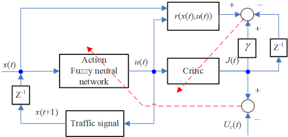
Adaptive model-free neuro-fuzzy system
1. Introduction
With the development of the economy and the degree of urbanization, urban traffic has increased rapidly. Traffic congestion, traffic safety and environmental problems are the most serious impacts of the traffic growth. Traffic signal control, which adjusts and reallocates traffic signal time, has been proven to significantly reduce traffic delays and bring considerable energy savings. There are different methods for traffic signal control. Wei et al. 1 and Xu et al. 2 investigated traffic signal control using various reinforcement learning algorithms. Tang et al. explored the potential of large language models for traffic control applications 3. Wei and Wang, Huang and Qu, and Jiang et al. designed different optimal control strategy 4,5,6. Wang explored the potential benefits of LoRa technology in traffic signal control 7. Zhang et al. studied traffic signal control in vehicular communication environment 8.
In the traffic signal arrangement problem, it is difficult to obtain a relatively good control effect by adopting a classical control strategy, such as the fixed time allocation method, because such controller cannot adjust with random time-varying traffic features. When the traffic volume changes, the performance of the fixed time mode is often weaker. Performance improvement can be achieved by constructing a signal control system with traffic flow feedback. Fuzzy logic has been employed in these control schemes since ancient times. Wei et al. used fuzzy logic and multi-objective genetic algorithm to carry out research to improve the flexibility of traffic signal control 9. Wu proposed optimization scheme of urban traffic light system which considers the dynamic characteristics of traffic conditions and can achieve more flexible and effective control strategies 10. Khan and Lai used fuzzy logic technology and image processing technology to design an intelligent traffic light controller with fuzzy logic control 11. Meepokgit and Wisayataksin combined deep Q-networks and fuzzy logic to optimize the waiting time of traffic lights and improve their efficiency 12. Most existing fuzzy controllers use static fuzzy algorithms. When the traffic environment changes, the fixed fuzzy rules are difficult to adjust automatically to make adaptive control decisions.
A neuro-fuzzy system is a combination of fuzzy systems and neural networks. Neuro-fuzzy systems can adjust fuzzy rules by training neural networks based on sample data. Fuzzy neural networks have been combined with advanced technologies to cope with the increasing complexity of urban traffic 13,14. In this way, knowledge for performance evaluation and knowledge for control policy selection work together as a unified framework 15,16,17. However, most existing neuro-fuzzy systems that adjust fuzzy parameters based on accumulated sample data struggle to adapt their parameters to non-stationary traffic conditions.
In recent years, with the development of artificial intelligence technology, reinforcement learning, and other algorithms have been applied to traffic signal control 18. Du et al. proposed an algorithm called Felight, which realizes traffic signal control with fairness awareness through a reinforcement learning method and solves the problem of ignoring vehicles waiting for a long time in traditional methods 19. Jiang et al. proposed a general reinforcement learning model without predefined scenes to automatically learn better traffic signal control strategies 20. Kuang et al. proposed a traffic signal control method based on reinforcement learning and state reduction, which generates a simplified Q-table and optimizes the complexity of the control algorithm 21. Raeis and Leon-Garcia proposed two traffic signal control methods based on deep reinforcement learning (DRL) to achieve these fairness and high throughput 22. Zhao et al., Jamil et al., and Kamal et al. uses digital twin technology and DRL model to reduce the travel time and vehicle emissions in the process of urban traffic signal control 23,24,25. Most existing reinforcement learning control algorithms require a traffic model and Q-table to learn, which limits their application. These algorithms are trained with randomly initialized parameters, which require more time to learn better results because of learning blindness.
Conversely, Werbos proposed a class of adaptive dynamic programming (ADP) as a new optimization technique that combines the concepts of dynamic programming and reinforcement learning 26. Adaptive critic learning design provides a new method for optimal control. Two artificial neural networks are employed: an action network and a critic network. The action network creates a control variable, and the critic network learns the performance target that the controller expects to achieve. These two neural networks cooperate to approximate the Hamilton–Jacobi–Bellman equation in the optimal control theory. Beginning with an arbitrarily selected action network rather than an optimal one, the adaptive learning process tends to the optimal solution under the guidance of the critic network with iteration performance. In one adaptive iteration, the required cost is the only parameter that needs to be known, and the optimal track information in classical reinforcement learning is not required. ADP can obtain an optimal control strategy under variable conditions 27. The conventional ADP methods have been used for traffic signal control 28,29.
2. Related Work
In this study, a model-free ADP (MFADP) is combined with a neuro-fuzzy system that can provide experiential knowledge for an action network. The proposed controller is denoted as model-free ADP-based neuro-fuzzy processor (MFADNFP). Simultaneously, the artificial bee colony (ABC) algorithm is employed for training the MFADNFP instead of the backpropagation gradient descent algorithm. Instead of classic neural network control, a neural fuzzy controller is used to provide prior expert knowledge to improve learning efficiency. The proposed controller can dynamically adjust the system parameters based on the enhanced signals (i.e., good/bad signals) to achieve proximity optimization results for multiple intersections. This allows the controller to learn the varying situations and reuse better solutions. This system is highly adaptable to time-varying traffic states and does not depend on offline processing that requires large amounts of historical data. The key works can be generalized as follows:
-
The proposed controller combines the advantages of the MFADP algorithm and a fuzzy system. MFADP algorithm provides self-learning optimization ability to adapt to varying traffic states and avoids the impact of a lack of an accurate time-varying traffic model.
-
The proposed controller applies a neuro-fuzzy system as the action network in the MFADP to generate control decisions. Thus, existing experience can be used to reduce the randomness in traditional ADP and accelerate optimization. The existing experience provided by the fuzzy membership function was optimized under the indicator of the MFADP adapting time-varying traffic states.
-
The ABC swarm algorithm is applied for the training of the MFADNFP so that the controller can adjust traffic signals in real time to meet variable traffic states.
The remainder of this paper is organized as follows. In Section 2, the main aim of the paper is briefly mentioned. In Section 3, traffic signal controller designed using ADP and neural fuzzy systems is discussed. The parameters of the neural fuzzy systems are adjusted using the ABC algorithm. Section 4 tests the controller proposed in the experiment with multiple intersections in the simulation. Section 5 analyses the controller’s capability in dealing with traffic signal control.
3. Design of Adaptive Dynamic Model-Free Neuro-Fuzzy Controller
In this section, we propose a traffic signal controller that combines model-free self-learning ability and expert expertise. We construct an MFADP framework to control traffic signals by applying neural fuzzy systems to the action network. The ABC algorithm is employed for training the ADP. The proposed controller, referred to as MFADNFP. At each intersection, the controller generates an optimal traffic signal plan with a real-time varying traffic state. To obtain the optimal area result, we applied a collaboration controller that received information from the adjacent intersection controller and decided on the approximate optimal signal scheme.
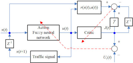
Fig. 1. Schematic diagram of the implementation of the MFADNFP.
3.1. The Overview of Controller
The traffic signal controller is processed using the MFADNFP. Fig. 1 shows a schematic of the proposed online learning control scheme. In Fig. 1, the input vector \(x(t)\) of the MFADNFP is selected as the number of vehicles in each phase. \(r(t)\) is the reinforcement feedback value. As illustrated in Fig. 1, dashed arrows denote parameter update paths, whereas solid arrows indicate data flow. In the conventional ADP methods, an artificial neural network is named action network. Before training, the parameters of this action network are randomly initialized, which leads to a longer training time and falls into a local optimal solution. We apply a neuro-fuzzy system as the action network to provide prior expert knowledge, which reduces blindness in training and improves learning efficiency.
A three-layer artificial neural network was used for the critic network. By training the critic network, the strategic utility or the cost-to-go function (the \(J\) in Bellman’s equation in dynamic programming) is approximated. The action network’s output signal is fed as an input to the critic network. The critic network performs the transfer learning operation in the controller; therefore, no track is required.
During the training of the critic network, no desired operation signal is required for optimization. The cost-to-go function \(J\) is only need for training the critic network.
3.2. Traffic Intersection Model
Figure 2 shows the case of two intersections, where each traffic intersection is numbered clockwise as N1, E1, S1, W1, N2, E2, S2, and W2 from left to right. The number of vehicles entered in each queue is given by the Poisson distribution with an average volume \(\lambda\), where \(\lambda\) is the ratio of the flow rate to the saturation flow rate.
To collect traffic data, pre-detector and rear-detector were installed on the stop and upstream lines, respectively. The rear-detector is used to count the number of vehicles entering the intersection: \(I_{i}(t)\) where \(i \in (\textrm{N1}, \textrm{E1}, \textrm{S1}, \textrm{W1}, \textrm{N2}, \textrm{E2}, \textrm{S2}, \textrm{W2})\). The pre-detector is used to count the number of vehicles dissipating the intersection \(Q_{i}(t)\). The distance between the pre-detector and rear-detector is defined as \(d\), the average length between two adjacent vehicles is defined as \(L\).
The maximum detectable value for each lane is limited by the following equation:
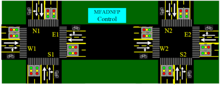
Fig. 2. A two-intersection case.
The number of vehicles in each lane \(i\) within \({\Delta t}\) can be calculated by the following:
The number of vehicles passing through the intersection within \({\Delta t}\) is defined:
The number of waiting vehicles follows with restriction:
Define the number of vehicles that arrive at any moment \(k\) as follows:
The number of vehicles entered within \({\Delta t}\) is defined as follows:
The number of vehicles on a lane within red light time \({\Delta t}\) is defined as following:
The sum waiting time in the red phase within \(\Delta t\) is defined as follows:
The number of vehicles on the lane within green signal time \({\Delta t}\) is defined as follows:
The sum waiting time in the green phase within \({\Delta t}\) is defined as follows:
The target which needs to be optimized is minimized \(T_{\mathit{waiting}}\) in Eq. 11.
3.3. The Action Network
In general, if vehicles in a phase are fewer, the green signal time will be short, but not shorter than the minimum green signal time (minGreen), so that the vehicle will have enough time to pass the intersection safely. For the same, if there are more vehicles need to pass, the green signal time will be longer, but it does not exceed the maximum green signal time (maxGreen), so that it does not exceed the driver’s mental patience.
A neural-fuzzy system is employed as action network. Control variable is generated based on four sets of data. These are \(\mathit{QN}\), \(\mathit{QE}\), \(\mathit{QS}\), and \(\mathit{QW}\), which correspond to the queue lengths in the north, east, south and west directions of the intersection. The states of action network are selected as follows:
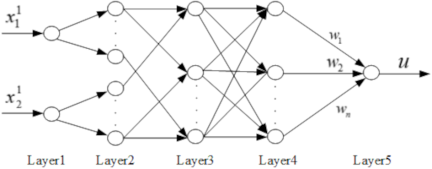
Fig. 3. The structure of the action network applied neuro-fuzzy system.
The output variable is defined as rate of extension for current green light phase. The structure for the neuro-fuzzy system is designed as Fig. 3. Input vector is defined as
The neuro-fuzzy network worked as action network has five layers structure. Node in the first layer is input node representing input linguistic variable. Node in the layer two is terminology node and serves as a membership function for representing each language variable. Each node in layer three is a rule node representing fuzzy logic rule. Node in layer four normalizes inputs in this layer. Node in layer five is the output. The following definitions were adopted in this paper. \(f_{i}^{(m)}\) is used to combine activation, information, or evidence from nodes in previous layer. This function provides input to node \(i\) in layer \(m\). \(o_{i}^{(m)}\) nodes a function which outputs an activation value based on inputs at node \(i\) in layer \(m\). The node functions in each layer are described below.
Layer 1: Node in the layer directly transfers the input value to the next layer.
Layer 2: Every node is used to perform membership functions. The bell-shaped function is employed for membership function.
Layer 3: Node in this layer works to prerequisite matching for executing fuzzy logic rule. It is necessary to perform the AND calculation which is employed the minimum operator in practice.
Layer 4: Nodes in this layer perform the normalization.
Layer 5: Node in this layer generates decision signal. Links connected to this layer and nodes work as the defuzzifier operation.
In this traffic signal controller, the following nine rules are selected as initial rules, where QLR and QLG represent the queue length in the phase with red or green light respectively. QLG and QLR are selected as \(x_1\) and \(x_2\) alternately according to traffic signal changing.
-
If QLG and QLR are all short, current green phase will be extended.
-
If QLG and QLR are short and medium, respectively, current green phase will be terminated.
-
If QLG and QLR are short and long, respectively, then terminate current green phase will be terminated.
-
If QLG and QLR are medium and short, respectively, current green phase will be extended.
-
If QLG and QLR are all medium, current green phase will be extended.
-
If QLG and QLR are medium and long, respectively, current green phase will be terminated.
-
If QLG and QLR are long and short, respectively, current green phase will be extended.
-
If QLG and QLR are long and medium, respectively, current green phase will be extended.
-
If QLG and QLR are all long, current green phase will be extended.
The principle of adjusting the action network is to indirectly reverse the error between the final goals \(U_c(t)\) and the cost-to-go function \(J\) from the critic network. Let
In the traffic signal control problem, the zero average waiting time will unable to achieve. Thus, the target of controller is to continuous decrease value. Thus, the minimum of the \(J(t-1)\) saved in early control cycle is chosen as \(U_{c}(t)\). the parameters of action network will be adjusted along decreasing direction of \(J(t)\) when \(e_{a}(t)\) is positive. The weights of action network will be adjusted to minimize the performance error value defined as follows:
3.4. The Critic Network
In this paper, following reinforcement function is chosen:
The structure of critic network is designed as a three-layer feedforward network which concludes input layer with three neurons, a hidden layer with five neurons, and one neuron output.
The critic network generates approximation of the discounted sum cost-to-go as output \(J\). The output \(J\) works as index to enhance the selection of better action. By optimizing action network and critic network, \(J\) will be reduced continuously and a smaller sum delay will be achieved. The prediction error of critical element is defined as
The target of critic network adjustment is to minimize the following objective function:
3.5. The Training of Action Network and Critic Network
In the conventional ADP, the backpropagation gradient descent algorithm is usually used for training of Action network and Critic network. However, there are some drawbacks. When the error surface is multi-peak, maybe the algorithm falls into the local minimum value. On the other hand, if the point reaches the output to the extremes before the convergence, saturation may occur. In this state, the weight will stop change because the derivative is too small.
Many global optimization methods have been proposed for training artificial neural networks to overcome the disadvantages of gradient algorithm, such as particle swarm optimization algorithm, differential evolution, genetic algorithms.
Karaboga has designed the ABC algorithm based on the behaving hunt behavior of honeybees and uses it for numerical optimization problems 30. It is simple, robust and the species group based on random optimization algorithm. The successful solution is related to finding a “batter solution” relatively fast. This is especially important for problems that need to be tackled in real time. Thus, the ABC algorithm is employed for proposed traffic signal controller to achieve optimal training with real-time traffic state.
Bees take direct tricks and dance in the nest. Their dance shows information about distance and direction. Bees will be foraging food sources based on this information. There are three types of honeybees: employ bees, bystanders and reconnaissance in the ABC algorithm. Food sources represent possible solutions for the problem that will be optimized. Each food source has only one employ bee. In the ABC algorithm, the development process is performed by bystanders and employ bees, and the search process is performed by reconnaissance.
In the first step, ABC randomly generates an initial population of \(\mathit{SN}\) solutions, where \(\mathit{SN}\) represents the size of population. Every solution \(\theta_{i}\) (\(i=1, 2, \dots, \mathit{SN}\)) is a \(D\)-dimensional vector. In this paper, we define a set of network parameters. Here, the number of parameters is defined as \(\mathit{WD}\). After initialization, the entire solution is circulated and repeated in the search processes.
Employ bees generate a rectification based on solutions in memory and tests the performance of new solution. When the performance of new solution is superior to the previous solution, the previous solution is replaced with the new one. On the contrary, previous solution will be kept. The employ bees could share the solution data and performance data with bystanders when they have finished once search process. Bystanders will appraise performance data collected from all employ bees, and select a solution with probability based on performances. Bystanders will produce a new location based on the selected solution, and test performance of this new location. The previous solution will be replaced when the performance of new location is better than the previous one.
Bystanders select a solution based on probability associated with this solution. The probability, \(P_{i}\), can be determined as follows:
In ABC algorithm, bees generate candidate solutions, \(v_{ij}\), with the following features from the old solution.
When performance of solution \(\theta_{i}\) will not be improved during preset training period, the employ bee who takes this solution will become a reconnaissance and solution \(\theta_{i}\) is abandoned. At the same time, bystanders will produce a new solution randomly. The abandoned solution is marked as \(\theta_{i} = [x_{i1}, x_{i2}, \dots, x_{iD}]\), the new solution will be generated as follows:
Greedy selection principle is used by bystanders to select better solution between the candidate and the old one.
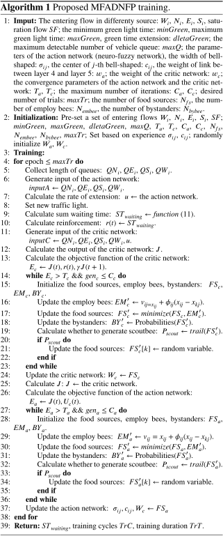
The overall algorithm of the proposed MFADNFP training is shown in Algorithm 1.
4. Simulations
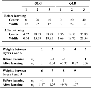
This section presents a simulation including two intersections. Some parameters in this simulation are chosen as following. The minGreen is set to 20 seconds, maxGreen is set to 120 seconds, green time extension is set to 20 seconds, and losing time of every phase is set to 1 second. The max detectable number of vehicle queue is set to 40. There are \(3\times 3=9\) logic rules full defined. Table 1 shows the initial values for the link weights between layer 4 and layer 5 in neuro-fuzzy network (the action network), and the center and width of each input membership function.
Table 1. Parameters of action network (neuro-fuzzy).
For training of the action network and the critic network using ABC algorithm, the convergence parameters of the action network and the critic network are set to 0.005 and 0.05, respectively. The maximum number of iterations are set to 200 and 150, respectively. The number of food sources, the number of employ bees and the number of bystanders is set 30 for everyone.
The logical flow of the simulation is shown in Algorithm 2.
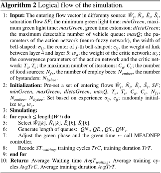
Table 2. Simulation results of case 1.
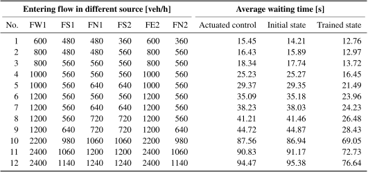
Table 3. Training times of case 1.
4.1. Case 1: Two Intersections
In this case, two intersections shown as Fig. 2 is chosen. A semi-actuated regulator is applied as a comparison. Semi-actuated regulator adjusts traffic signal time based on the comparison of traffic intensity between non-actuated street (usually the major street) and other actuated streets. Some parameters in semi-actuated regulator, such as minGreen, maxGreen, and green time extension, are set as above. The green signal of the main phase (east-west phase) will be interrupted until starting of the secondary phase (north-south phase). When the secondary phase is no longer urgent, main phase will be set green signal again.
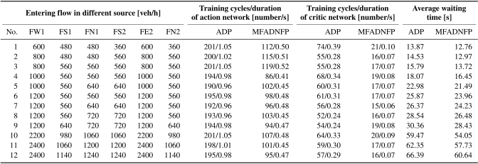
Simulation will execute ten times, and each execution includes 1000 traffic signal cycles. The average value of ten execution is chosen for comparison. The simulations run in the environment with 2.3 GHz CPU and 64 GB memory. The optimized control decision is obtained within 0.1–0.5 seconds. The parameters before and after optimization in neuro-fuzzy network (the action network) of proposed controller are listed in Table 1. Table 2 summarizes the simulation results of the proposed control algorithm under various traffic-flow scenarios, including both peak and off-peak periods, with semi-actuated algorithm results provided for comparison. Relative to the semi-actuated algorithm, the proposed scheme reduces average waiting time by 17%–37% relative to the semi-actuated controller. In addition, The simulation data in Table 2 indicate that optimizing the fuzzy rules reduces the average waiting time by 10%–37% relative to the initial parameter set. Simulation results demonstrate that the proposed control algorithm autonomously adjusts its fuzzy-rule parameters through online learning in response to evolving traffic conditions, achieving a consistent reduction in average waiting time and thereby exhibiting robust adaptability to time-varying traffic flows.
The training times of action network and critical network and the average waiting time under different traffic flows are compared. The simulation results are listed in Table 3. For the training of action network, proposed MFADNFP algorithm reduces training time about 60% and decreasing waiting time about 6% compared with ADP based on backpropagation gradient descent algorithm. For the training of critical module, proposed algorithm reduces about 70% than ADP based on backpropagation gradient descent algorithm. Because the performance of the optimized parameters obtained by the two methods is similar, the control effect (average vehicle waiting time) is approximately equal. This show that MFADNFP algorithm can achieve optimal control quickly and avoid proposed controller trapped at local minima.
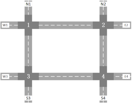
Fig. 4. The traffic network structure with four intersections.
4.2. Case 2: Four Intersections
In this section, a case of two traffic intersections is simulated. Fig. 4 shows the traffic network structure to be studied, where we number each traffic intersection from left to right and from top to bottom. For ease of illustration, only through traffic at the intersection is considered; turning movements are ignored. At this case, the source of vehicles entering the region can be regarded as N1, N2, S3, S4, W1, W3, E1, and E4, and each intersection comprises two through phases: north-south phase and east-west, that need phase to be controlled. The DRL is tested for comparison. Each scenario is simulated over ten independent runs, and each execution includes 1000 traffic signal cycles. The averaged metrics across the ten runs are reported.
Table 4 presents the simulation results of four intersections case. When the traffic flow in all directions of a intersection is relatively balanced (Nos.1, 8, and 9), the initial fuzzy rule parameters that needed to be optimized in the proposed MFADNFP algorithm is relatively concentrated. Therefore, the optimization training speed is faster, reaching the preset convergence criteria in about 100 iterations. When the traffic flow in different directions of a intersection becomes more unbalanced, the range of fuzzy rule parameters that need to be adjusted increases, and the number of algorithm optimization training iterations correspondingly increases. In contrast, the DRL network has a larger scale and far more parameters than MFADNFP. Moreover, the initial parameters of the network are randomly generated, resulting in a training iteration count that is approximately 3.5 times that of MFADNFP.
When running in the same environment as case 1, as the number of simulated intersections increases, the average number of training iterations remains relatively stable. However, limited by the computational capacity, the average training time increases.
In terms of control effectiveness, due to the initial fuzzy rule experience of MFADNFP, the initial exploration process is relatively short. In the simulation case, the overall average waiting time increases from 12.76 s to 63.74 s with the increase of traffic flow. However, due to the fact that the DRL algorithm is optimized based on a large number of random parameters, the training cycle to reach the optimization goal is longer, resulting in an increase in average waiting time by 13%–23%.
Figure 5 illustrates, for different intersections and under varying traffic volumes, the evolution of vehicle queue lengths together with the corresponding traffic-signal changes. Each intersection is represented by a distinct line style denoting the queue length (\(\mathit{QW}_{i}\), \(\mathit{QE}_{i}\), \(\mathit{QN}_{i}\), and \(\mathit{QS}_{i}\)) on its four approaches (west, east, south, and north). The color of each queue segment indicates the current signal phase at that approach. It can be seen that, as queue lengths in different directions vary, the green time for the corresponding phase is adjusted accordingly, achieving an optimized and coordinated response to the prevailing demand for each movement.
Table 4. Simulation results of case 2.
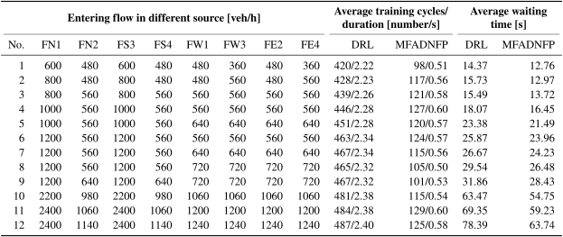
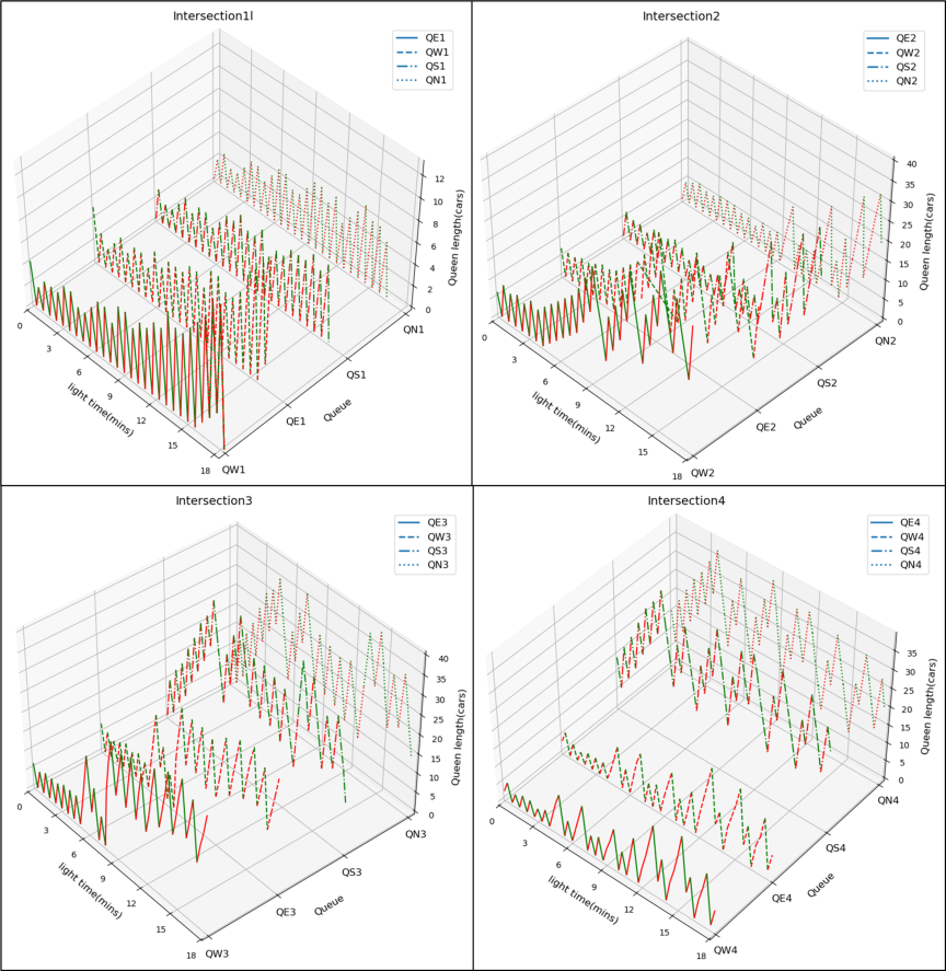
Fig. 5. The correspondence between queue state and signal state.
5. Conclusion
The actual traffic environment has remarkable time variability and randomness characteristics. The traditional fixed time plans cannot well adapt to the changing traffic conditions. At the same time, the classic traffic model makes some assumptions and restrictions, which cannot adapt to randomness well. This paper presented a controller which combines a neuro-fuzzy system and MFADP. This MFADP does not require a traffic model and can provide self-learning optimization ability. So that the proposed controller can respond to fluctuated traffic state well through continuous learning based on evaluation index.
In the proposed controller, a neuro-fuzzy network is worked as the action network in MFADP; thus the proposed controller exhibits significantly reduced exploration inefficiency and achieves minimal average wait time more quickly based on experience supplied by the fuzzy rule. At the same time, the initial experience will be adjusted under MFADP indication to adapt to varying traffic states. Furthermore, the ABC algorithm is applied for training the action and critic networks. The controller meets the real-time requirement for traffic signal control by generating control decisions quickly based on ability in achieving optimal control quickly and avoiding the proposed controller trapped at local minima.
The action network requires longer training time than the critic network because its convergence threshold is more stringent. Simulation results show the proposed controller achieves a little lower average waiting time using shorter training time compared to other methods. Future research will enhance the robustness of controllers to cope with the impact of traffic emergencies in other traffic scenarios (sudden surges, abnormal events, etc.). We will improve the controller design to adapt to more scenarios. The convergence and stability of the algorithm will also be studied.
Acknowledgments
This research was funded by high-level talents and key scientific research projects of Nanjing Vocational Institute of Transport Technology; Jiangsu Transportation Science and Technology project, grant numbers JG2521, JZ2408, and JT2024YB070.
- [1] H. Wei, G. Zheng, V. Gayah, and Z. Li, “Recent advances in reinforcement learning for traffic signal control: A survey of models and evaluation,” ACM SIGKDD Explorations Newsletter, Vol.22, No.2, pp. 12-18, 2021. https://doi.org/10.1145/3447556.3447565
- [2] B. Xu, Y. Wang, Z. Wang, H. Jia, and Z. Lu, “Hierarchically and cooperatively learning traffic signal control,” Proc. of the AAAI Conf. on Artificial Intelligence, Vol.35, No.1, pp. 669-677, 2021. https://doi.org/10.1609/aaai.v35i1.16147
- [3] Y. Tang, X. Dai, and Y. Lv, “Large language model-assisted arterial traffic signal control,” IEEE J. of Radio Frequency Identification, Vol.8, pp. 322-326, 2024. https://doi.org/10.1109/jrfid.2024.3384289
- [4] W. Wei and M. Wang, “Research on traffic signal control based on intelligence techniques,” Proc. of the 2003 IEEE Int. Conf. on Intelligent Transportation Systems, Vol.1, pp. 892-896, 2003. https://doi.org/10.1109/itsc.2003.1252078
- [5] L. Huang and X. Qu, “Improving traffic signal control operations using proximal policy optimization,” IET Intelligent Transport Systems, Vol.17, No.3, pp. 592-605, 2023. https://doi.org/10.1049/itr2.12286
- [6] C.-Y. Jiang, X.-M. Hu, and W.-N. Chen, “An urban traffic signal control system based on traffic flow prediction,” 2021 13th Int. Conf. on Advanced Computational Intelligence, pp. 259-265, 2021. https://doi.org/10.1109/icaci52617.2021.9435905
- [7] F. C. Wang, “Design and implementation of intelligent traffic signal light control system based on LoRa technology,” Applied and Computational Engineering, Vol.117, pp. 107-113, 2025. https://doi.org/10.54254/2755-2721/2025.20314
- [8] Y. Zhang et al., “An occupancy-based adaptive signal control for a congested signalized intersection in the low CV penetration environment,” J. of Advanced Transportation, Vol.2022, Article No.4745879, 2022. https://doi.org/10.1155/2022/4745879
- [9] W. Wei, Y. Zhang, J. B. Mbede, Z. Zhang, and J. Song, “Traffic signal control using fuzzy logic and MOGA,” 2001 IEEE Int. Conf. on Systems, Man and Cybernetics, e-Systems and e-Man for Cybernetics in Cyberspace, Vol.2, pp. 1335-1340, 2001. https://doi.org/10.1109/ICSMC.2001.973106
- [10] Y. Wu, “Enhancing urban traffic flow through fuzzy logic-based signal light control optimization,” Int. J. of e-Collaboration, Vol.20, No.1, 2024. https://doi.org/10.4018/ijec.358746
- [11] B. A. Khan and N. S. Lai, “An advanced fuzzy logic based traffic controller,” Int. J. of Innovation in the Digital Economy, Vol.5, No.1, pp. 31-40, 2014. https://doi.org/10.4018/ijide.2014010103
- [12] T. Meepokgit and S. Wisayataksin, “Traffic signal control with state-optimizing deep reinforcement learning and fuzzy logic,” Applied Sciences, Vol.14, No.17, Article No.7908, 2024. https://doi.org/10.3390/app14177908
- [13] E. Bingham, “Reinforcement learning in neurofuzzy traffic signal control,” European J. of Operational Research, Vol.131, No.2, pp. 232-241, 2001. https://doi.org/10.1016/s0377-2217(00)00123-5
- [14] M. C. Choy, D. Srinivasan, and R. L. Cheu, “Cooperative, hybrid agent architecture for real-time traffic signal control,” IEEE Trans. on Systems, Man, and Cybernetics – Part A: Systems and Humans, Vol.33, No.5, pp. 597-607, 2003. https://doi.org/10.1109/tsmca.2003.817394
- [15] Ö. N. Kenger and E. Özceylan, “Fuzzy min–max neural networks: A bibliometric and social network analysis,” Neural Computing and Applications, Vol.35, No.7, pp. 5081-5111, 2023. https://doi.org/10.1007/s00521-023-08267-9
- [16] C. Wang, X. Lv, M. Shao, Y. Qian, and Y. Zhang, “A novel fuzzy hierarchical fusion attention convolution neural network for medical image super-resolution reconstruction,” Information Sciences, Vol.622, pp. 424-436, 2023. https://doi.org/10.1016/j.ins.2022.11.140
- [17] J. Dai et al., “A fuzzy adaptive zeroing neural network model with event-triggered control for time-varying matrix inversion,” IEEE Trans. on Fuzzy Systems, Vol.31, No.11, pp. 3974-3983, 2023. https://doi.org/10.1109/tfuzz.2023.3272653
- [18] H. Zhao, C. Dong, J. Cao, and Q. Chen, “A survey on deep reinforcement learning approaches for traffic signal control,” Engineering Applications of Artificial Intelligence, Vol.133, Part A, Article No.108100, 2024. https://doi.org/10.1016/j.engappai.2024.108100
- [19] X. Du et al., “FELight: Fairness-aware traffic signal control via sample-efficient reinforcement learning,” IEEE Trans. on Knowledge and Data Engineering, Vol.36, No.9, pp. 4678-4692, 2024. https://doi.org/10.1109/TKDE.2024.3376745
- [20] H. Jiang et al., “A general scenario-agnostic reinforcement learning for traffic signal control,” IEEE Trans. on Intelligent Transportation Systems, Vol.25, No.9, pp. 11330-11344, 2024. https://doi.org/10.1109/tits.2024.3377106
- [21] L. Kuang, J. Zheng, K. Li, and H. Gao, “Intelligent traffic signal control based on reinforcement learning with state reduction for smart cities,” ACM Trans. on Internet Technology, Vol.21, No.4, Article No.102, 2021. https://doi.org/10.1145/3418682
- [22] M. Raeis and A. Leon-Garcia, “A deep reinforcement learning approach for fair traffic signal control,” arXiv:2107.10146, 2021. https://doi.org/10.48550/arXiv.2107.10146
- [23] Z. Zhao, K. Wang, Y. Wang, and X. Liang, “Enhancing traffic signal control with composite deep intelligence,” Expert Systems with Applications, Vol.244, Article No.123020, 2024. https://doi.org/10.1016/j.eswa.2023.123020
- [24] A. R. M. Jamil, K. K. Ganguly, and N. Nower, “Adaptive traffic signal control system using composite reward architecture based deep reinforcement learning,” IET Intelligent Transport Systems, Vol.14, No.14, pp. 2030-2041, 2020. https://doi.org/10.1049/iet-its.2020.0443
- [25] H. Kamal, W. Yánez, S. Hassan, and D. Sobhy, “Digital-twin-based deep reinforcement learning approach for adaptive traffic signal control,” IEEE Internet of Things J., Vol.11, No.12, pp. 21946-21953, 2024. https://doi.org/10.1109/jiot.2024.3377600
- [26] P. J. Werbos, “Approximate dynamic programming for real-time control and neural modeling,” D. A. White and D. A. Sofge (Eds.), “Handbook of Intelligent Control: Neural, Fuzzy, and Adaptive Approaches,” pp. 493-525, Van Nostrand Reinhold, 1992.
- [27] D. Wang, N. Gao, D. Liu, J. Li, and F. L. Lewis, “Recent progress in reinforcement learning and adaptive dynamic programming for advanced control applications,” IEEE/CAA J. of Automatica Sinica, Vol.11, No.1, pp. 18-36, 2024. https://doi.org/10.1109/JAS.2023.123843
- [28] C. Cai, “An approximate dynamic programming strategy for responsive traffic signal control,” 2007 IEEE Int. Symp. on Approximate Dynamic Programming and Reinforcement Learning, pp. 303-310, 2007. https://doi.org/10.1109/ADPRL.2007.368203
- [29] T. Li, D. Zhao, and J. Yi, “Application of ADP to intersection signal control,” Proc. of the 4th Int. Symp. on Neutral Networks, Part 1, pp. 374-379, 2007. https://doi.org/10.1007/978-3-540-72383-7_44
- [30] D. Karaboga, “An idea based on honey bee swarm for numerical optimization,” Technical Report-TR 06, Erciyes University, 2005.
This article is published under a Creative Commons Attribution-NoDerivatives 4.0 Internationa License.