
Research Paper:
A Corporate Financial Analysis Framework Based on RFECV-PRF Feature Selection and GA-LightGBM
Cui Hu†
Chongqing College of Finance and Economics
No.1888 Honghe South Road, Yongchuan District, Chongqing 402160, China
†Corresponding author

Financial fraud in listed companies has attracted increasing academic attention due to its severe implications for investors and market stability. Traditional methods for detecting fraudulent financial statements have proven insufficient in addressing the growing complexity and volume of financial data. This study proposes a novel hybrid model combining recursive feature elimination with cross-validation and parallel random forest (RFECV-PRF) for feature selection and a genetic algorithm-optimized LightGBM (GA-LightGBM) for financial fraud detection. The RFECV-PRF method effectively evaluates feature importance and selects the optimal subset of financial indicators, while the GA-LightGBM model enhances prediction accuracy and efficiency through global optimization of hyperparameters. Empirical tests using data from five industries—energy, materials, industrials, information technology, and healthcare—demonstrated significant improvements in classification accuracy, precision, recall, and F1 scores. The proposed framework outperforms traditional machine learning approaches such as random forest and XGBoost, achieving superior results in detecting fraudulent financial activities. This research highlights the potential of integrating advanced feature selection methods with optimized machine learning models to address the challenges of financial fraud detection and improve the reliability of corporate financial reporting.
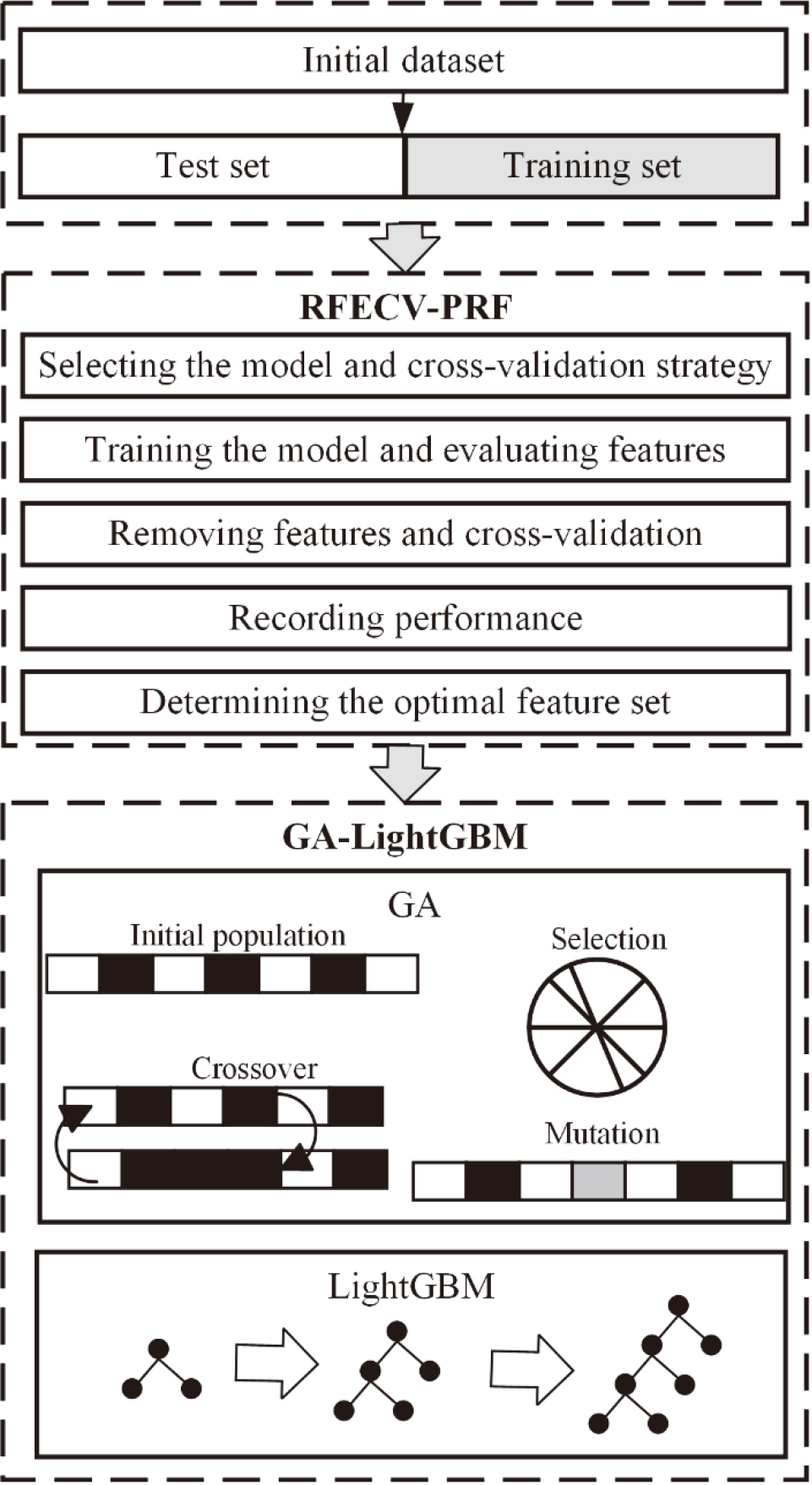
RFECV-PRF-GA-LightGBM model framework
1. Introduction
Financial statement fraud has gradually become a focal point of academic attention. This type of fraud includes inflating assets, revenues, and profits or underestimating liabilities and losses 1,2. Financial fraud can cause significant losses for investors, undermine the efficient allocation of resources, and disrupt the normal functioning of markets 3. In 2019, General Electric (GE) misled investors through a series of disclosure errors, leading to investments totaling $38 billion, which accounted for more than 40% of GE’s market value 4. Despite increased regulatory oversight and efforts by governments and authorities to combat corporate financial fraud, the phenomenon persists. Nearly 30% of companies worldwide engage in financial manipulation. Among the most common fraudulent techniques are the fabrication of revenues and assets 5. Traditional methods of observation, inquiry, and basic financial statement analysis are inefficient and no longer suffice to meet the current demands for financial analysis. Thus, there is a need for more intelligent financial statement analysis and predictive models.
Financial statement fraud is one of the primary means and manifestations of corporate financial fraud in publicly listed companies 6. Financial statements are standardized documents that reflect a company’s financial condition, operational results, and cash flows. Their purpose is to help investors, creditors, and other stakeholders assess the company’s performance and financial health. In addition, financial statements often include explanatory notes from management, aimed at clarifying the company’s operational performance and forecasting potential future challenges. These reports provide a comprehensive picture of the company’s financial condition and achievements, which is crucial for evaluating its financing potential. Financial statement fraud typically aims to present a company’s financial position as better than it truly is, thereby misleading investors and stakeholders and affecting the company’s stock price, credit rating, or ability to secure loans 7.
Data mining is a commonly used method for detecting financial statement fraud, which encompasses statistical, machine learning, mathematical, and artificial intelligence techniques to extract meaningful information from the given data 6. Data mining identifies financial statement fraud by employing principles such as classification, clustering, anomaly detection, and regression. Support vector machine (SVM) achieves classification by finding a hyperplane that maximizes the margin, separating data points of different categories, where the maximization refers to the largest distance between the closest data points (i.e., support vectors) on either side of the decision boundary 8. Sundarkumar et al. 9 proposed an undersampling method based on one-class SVM for customer churn prediction and insurance fraud detection. By merging the support vectors extracted from the major class samples with the minority class samples, a balanced dataset was created, significantly improving classifier performance. Deng 10 developed an SVM-based model for detecting financial statement fraud to identify fraudulent financial reports. They used 44 fraud samples and 44 non-fraud samples from Chinese listed companies between 1999 and 2002 as a training dataset, and 73 fraud samples and 99 non-fraud samples from 2003 to 2006 as a test dataset. The model, trained and applied to the test dataset, produced promising results.
Fuzzy logic (FL) simulates the way humans process uncertainty and ambiguity by allowing variables to take values within a certain range, rather than adhering to strict binary oppositions (true or false) 11. FL has been employed to detect vehicle insurance fraud. Supraja and Saritha 12 modeled attributes such as driver age and vehicle age using fuzzy logic and “IF-THEN” rules, enabling the system to predict insurance fraud occurrences. This method efficiently handles high-dimensional data, with high accuracy and low time complexity, and the results are easy to interpret. Saeed and Hagras 13 simulated human fuzzy reasoning to handle uncertain and ambiguous data, generating “IF-THEN” rules from transaction data such as amount, time, and transaction type. Type-2 fuzzy logic was applied to address ambiguous cases, and the rule base was updated regularly to accommodate new fraud patterns, offering high transparency and facilitating expert analysis for financial fraud detection.
Machine learning algorithms, as the most important data mining tools for discovering and extracting hidden relationships and truths in large datasets, have become vital methods for identifying financial statement fraud 14. To ensure that the designed systems can distinguish between fraudulent and non-fraudulent cases, 15 evaluated various machine learning methods, with the artificial neural network model showing the best performance in terms of accuracy and area under the ROC curve (AUC), particularly in predicting false positives and missed reports. Hajek 16 focused on the interpretability of detected fraud behaviors, reducing the search space through feature selection and optimizing fuzzy rule bases using both evolutionary and non-evolutionary algorithms to enhance prediction accuracy and interpretability. Lokanan et al. 17 used Mahalanobis distance to detect anomalies in financial statements of listed companies in Vietnam. Their analysis of data from 937 companies and 24 financial indicators found that while most companies’ financial statements were reliable, about a quarter showed significant anomalies. Furthermore, other scholars have utilized methods such as \(k\)-nearest neighbors 18, random forest 19, decision trees 20, CatBoost 21, and Bayesian networks 22 for financial fraud detection. In recent years, researchers have also proposed using techniques like knowledge graphs 1, systematic reviews 23, and bag-of-words models 24 for detecting financial fraud.
In summary, machine learning has become the mainstream method for identifying financial fraud in enterprises. However, as financial data continues to grow, the volume of data that needs to be identified and analyzed is expanding exponentially. Traditional machine learning models are no longer sufficient to meet the current requirements for high real-time performance and accuracy. To address these issues, this paper proposes a lightweight gradient boosting machine (LightGBM) model, which is optimized through parallel random forest (PRF) 25 and recursive feature elimination with cross-validation (RFECV) for feature selection, along with genetic algorithms (GA) for parameter optimization. This model can effectively identify financial fraud-related indicators in corporate data.
2. Methodology
2.1. RFECV-PRF Algorithm
Recursive feature elimination (RFE) is commonly used in feature selection tasks. It works by recursively removing the least important features, followed by training and evaluating the model on the remaining features, until the desired number of features is achieved or a performance criterion is met 26.
The RFECV method selects a key subset of features by recursively eliminating those with minimal contribution to the model, and uses cross-validation to assess performance at different feature set sizes in order to determine the optimal subset size. The core steps include recursive ranking of feature importance, stepwise removal, and cross-validation to select the feature set with the highest average performance. PRF generates multiple decision trees in parallel during each feature subset iteration, utilizing a parallel computing framework to simultaneously train and validate the model on each fold of cross-validation data. This approach maintains the RFECV’s recursive elimination mechanism while reducing the computational complexity of feature importance evaluation and model validation from linear to logarithmic scale. The basic process of PRF-enhanced RFECV is as follows:
-
(1)
Training the model and calculating the root mean square error: For the current feature subset \(S_k\), we train a random forest model using cross-validation and compute the root mean square error (RMSE) to evaluate the model’s performance:
\begin{equation} \label{eq:1} \textrm{RMSE}\left(S_k\right)=\sqrt{\dfrac{1}{n}\sum_{i=1}^n \left(y_i -\hat{y}\left(S_k\right)\right)^2}. \end{equation}In this context, \(S_k\) represents the feature subset in the \(k\)-th round of RFE, \(y_i\) denotes the true values, and \(\hat{y}\,(S_k)\) refers to the predicted values obtained using the feature subset \(S_k\).
-
(2)
Feature elimination: In each iteration, the feature with the smallest contribution is removed based on the model’s feature importance value \(I_j\). The feature importance \(I_j\) can be computed using the formula for the cumulative impurity reduction in the random forest:
\begin{equation} \label{eq:2} I_j=\sum_{t=1}^T \sum_{s\in S(j,t)} \Delta I(s,t). \end{equation}Then, the feature with the smallest \(I_j\) value is removed.
-
(3)
As the RFE progresses, the number of features is gradually reduced, and the RMSE of the model is calculated after each iteration. Ultimately, by comparing the RMSE values of all feature subsets, the subset with the smallest RMSE is selected as the final feature set:
\begin{equation} \label{eq:3} S^{\ast}=\underset{S_k}{\arg\min}\, \textrm{RMSE}\left(S_k\right). \end{equation}
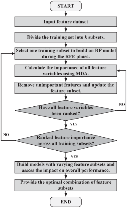
Fig. 1. Main steps of RFECV-RF.
The key steps of this process are shown in Fig. 1, where MDA stands for mean decrease accuracy, which is used to assess the importance of the features in the RF model. The formula for MDA is as follows:
2.2. GA-LightGBM Algorithm
LightGBM is a machine learning method based on the gradient boosting framework, which incorporates several novel techniques to optimize training efficiency and prediction accuracy. Compared to conventional gradient boosting decision tree (GBDT) algorithms, LightGBM demonstrates superior performance when handling large datasets and complex features 27. GBDT is an additive ensemble model that uses classification and regression trees as base learners. Let \(X=x_i\), \({y_i}_{i=1}^M\) represent the training set, consisting of \(M\) samples, \(x_i\in {K}^n\) denote the feature vector, and \(y_i\in {K}\) represent the target values. The core principle of GBDT is to minimize the loss function \(L(y,F(x))\), which quantifies the difference between the predicted and actual values.
The loss function is defined as follows:
In each iteration, the negative gradient of the current prediction \(-\partial L(y,F_{k-1}(x))/\partial F_{k-1}(x)\) is used to fit a decision tree \(h_k(x)\). The residual can be expressed as:
The training objective of the \(k\)-th decision tree is to minimize the loss function \(L(y_i,F_{k-1}(x_i)+h_k(x_i))\). After \(k\) iterations, the predicted value \(F_k(x)\) is the weighted sum of the predictions from all decision trees, with the weights controlled by the learning rate \(\gamma_k\):
Here, \(J_k\) represents the number of leaf nodes in the decision tree, and \(I(x\in R_{jk})\) is the indicator function. The final predicted value \(F(x)\) is the weighted sum of the predictions from all decision trees:
LightGBM introduces several improvements over traditional GBDT in multiple aspects. It employs a histogram-based decision tree algorithm, which discretizes continuous features into discrete intervals, significantly reducing memory usage and computational complexity, making it particularly suitable for large-scale datasets. Additionally, LightGBM uses a leaf-wise growth strategy, which is more efficient than the traditional level-wise approach but may lead to overfitting, requiring hyperparameter tuning. It also supports direct handling of categorical features without the need for manual encoding. Furthermore, LightGBM is capable of distributed computing, enabling efficient processing of large datasets.
In LightGBM, hyperparameters are typically tuned using grid search. In contrast, GA-LightGBM optimizes hyperparameters using a GA, which can identify the optimal parameter combination. The process of constructing the GA-LightGBM algorithm involves the following key steps:
-
(1)
Initial population generation: The initial population is created by encoding each randomly selected combination of hyperparameters. During the generation of the initial population, the L1 regularization parameter (lambda_l) and the L2 regularization parameter (lambda_2) are included in the hyperparameter combinations.
-
(2)
Model training and performance evaluation: The LightGBM model is trained using the hyperparameter combinations that include the L1 and L2 regularization parameters. The model’s performance is evaluated on the test set, with the mean absolute percentage error (MAPE) used as the performance metric.
-
(3)
Fitness calculation: The fitness value for each individual is calculated based on the MAPE value, where fitness is defined as the reciprocal of MAPE.
-
(4)
Natural selection and genetic operations: Individuals with lower fitness values are eliminated through a roulette-wheel natural selection algorithm. The remaining individuals undergo crossover and mutation operations to generate a new population.
-
(5)
Iteration: The updated population is used for model prediction. Repeat Steps 2 to 4 until the preset number of iterations is reached (as shown in Table 1).
-
(6)
Output results: The optimal individual, corresponding to the best hyperparameter combination, is identified, yielding the highest accuracy result from the GA-LightGBM algorithm 28.
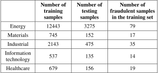
Table 1. Experimental data.
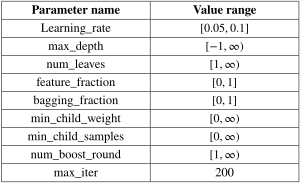
The basic information of the initialization parameters for GA-LightGBM is shown in Table 2.
Table 2. Basic information of parameters.
2.3. Overall Model Theory Construction
Therefore, this paper adopts a financial fraud detection model based on GA-LightGBM with RFECV-PRF feature selection, which consists of two main parts. The modeling steps are as follows:
-
Feature selection with RFECV-PRF: The preprocessed full-feature training data is input into RFECV-PRF to uncover the relationships between features and evaluate their importance. The RFECV automatically selects the optimal feature subset, excluding irrelevant or low-impact features. This helps avoid issues such as excessive computational load and low classification accuracy due to feature redundancy.
-
Hyperparameter optimization with GA: The optimal feature subset is fed into LightGBM. Given the diverse parameter combinations in LightGBM, a GA is used for global optimization of the parameter combinations, identifying the most effective set of parameters.
-
Prediction with the optimized model: The optimal feature data from the test set is input into the LightGBM model with the optimal parameter combination obtained in Step 2 to make predictions.
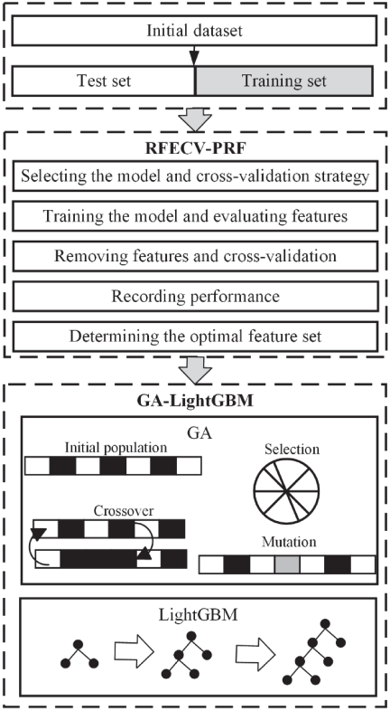
Fig. 2. Model framework.
The framework of the GA-LightGBM model based on RFECV-PRF feature selection is shown in Fig. 2.
To effectively evaluate the model’s performance, three metrics are introduced to assess and validate its effectiveness:
Accuracy indicates the proportion of correctly predicted samples in comparison to the total predictions made. It measures how many of the predicted results match the actual outcomes:
Precision refers to the proportion of true positive samples among all the samples predicted as positive:
Recall refers to the proportion of true positive samples among all the actual positive samples:
The F1 score is the harmonic mean of precision and recall, providing a balanced evaluation of the classification model’s accuracy.
The ROC curve is a graph with the false positive rate (FPR) on the \(x\)-axis and the true positive rate (TPR) on the \(y\)-axis. As the threshold changes, the FPR and TPR of the model vary, forming the ROC curve. By calculating the area under the ROC curve, known as the AUC value, the performance of the ROC curve can be evaluated. The AUC value ranges from 0.5 to 1, with a larger value indicating better model performance.
3. Simulation Experiment
3.1. Experimental Data
The data used in this study is sourced from a corporate violation database compiled by a certain company. The corporate data samples are categorized into two groups: fraudulent samples and non-fraudulent samples. Financial fraud is further divided into three major categories: fabricated finances, false reporting, and significant omissions. The experimental data is shown in Table 1.
3.2. Experimental Procedure
Due to the different dimensions and units of the data, which can affect the results of subsequent data analysis, it is necessary to normalize the numerical indicators. This ensures that the indicators are scaled within the range \([0,1]\). The specific normalization process is as follows:
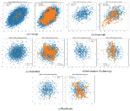
Fig. 3. Comparison before and after SMOTE processing.
In the equation, \(\max(x)\) represents the maximum value of indicator \(x\), and \(\min(x)\) represents the minimum value of \(x\).
Data balancing processing: Considering the potential class imbalance in the dataset (i.e., financial fraud samples are fewer compared to non-fraud samples), we applied the synthetic minority oversampling technique (SMOTE) method to oversample the minority class (financial fraud) in the training set. SMOTE balances the dataset by generating new minority class samples, ensuring that the training data for each industry is more balanced, thereby reducing the negative impact of class imbalance on model training. Fig. 3 illustrates the sample distribution across different industries before and after SMOTE processing.
To eliminate irrelevant features, avoid overfitting, and improve evaluation accuracy, after data normalization, the PRF and RFECV method is used to assess feature importance and construct the optimal feature subset. After constructing the optimal subset from the original 102 features across the five industries, the optimal feature subset for each industry is shown in Tables 3–7.
Table 3. Feature selection for the energy industry.
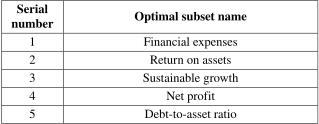
Table 4. Feature selection for the materials industry.
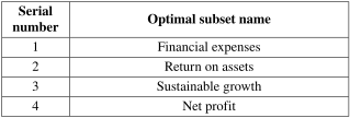
Table 5. Feature selection for the industrial industry.
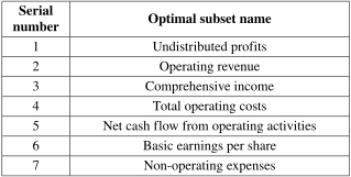
Table 6. Feature selection for the information technology industry.
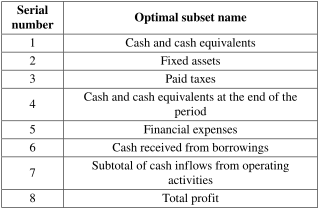
Table 7. Feature selection for the healthcare industry.
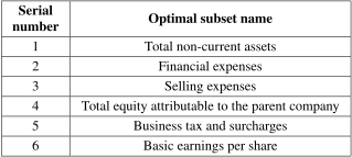
Table 8. Comparison of the effects of LightGBM before and after using RFECV-PRF.
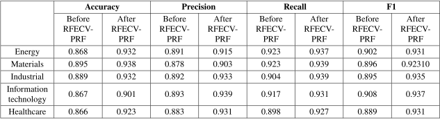
Table 9. Comparison of simulation experiments between LightGBM and GA-LightGBM.
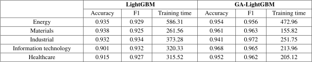
Table 10. Evaluation results of different models.
The LightGBM model is used to validate the accuracy and efficiency of the evaluation before and after feature selection. As shown in Table 8, when RFECV-PRF is not used for feature selection, the evaluation metrics for each industry through LightGBM are lower than those after feature selection. From the results in Table 8, taking the energy industry as an example, after feature selection, the accuracy increases from 0.868 to 0.932, while the precision rises from 0.891 to 0.915; recall and F1 score also show improvements.
After feature selection, the LightGBM model shows improved performance across all five industries, as presented in Table 8. Specifically, accuracy increases from 0.868 to 0.932 in the energy industry, from 0.895 to 0.938 in the materials industry, from 0.889 to 0.932 in the industrial industry, from 0.867 to 0.901 in the information technology industry, and from 0.866 to 0.923 in the healthcare industry. Precision, recall, and F1 score also improve after RFECV-PRF feature selection, indicating that the selected feature subsets effectively enhance the classification performance.
The comparison between LightGBM and GA-LightGBM in Table 9 further shows that GA-based hyperparameter optimization improves both prediction performance and training efficiency. For example, in the energy industry, accuracy increases from 0.935 to 0.954, while the F1 score rises from 0.929 to 0.956, and the training time decreases from 586.31 to 472.96. Similar improvements are observed in the materials, industrial, information technology, and healthcare industries, demonstrating that GA-LightGBM achieves better overall performance than the standard LightGBM model.
To eliminate the impact of subjective factors on model evaluation performance, GA is used to select the parameters for the LightGBM model. Both LightGBM and GA-LightGBM models are used to evaluate the performance metrics of several industries that have already undergone feature selection. The results are shown in Table 9.
The comparison of simulation experiments between LightGBM and GA-LightGBM, as shown in Table 9, indicates that GA-LightGBM outperforms the standard LightGBM model in all industries. For example, in the energy industry, the accuracy of GA-LightGBM increases from 0.93421 to 0.95768, and the F1 score rises from 0.92763 to 0.95824. In the materials industry, accuracy improves from 0.93645 to 0.95978, and the F1 score increases from 0.92310 to 0.96562. Similarly, in the industrial sector, GA-LightGBM achieves a higher accuracy of 0.96426 compared to 0.93090 with LightGBM, and the F1 score improves from 0.93603 to 0.97512. The information technology and healthcare industries also show improvements in both accuracy and F1 score with GA-LightGBM. These results demonstrate that the use of GA for hyperparameter optimization significantly enhances the model’s performance across all industries.
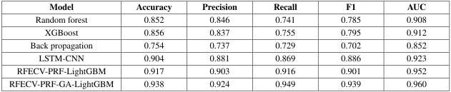
To validate the performance of the RFECV-PRF feature selection combined with the GA-LightGBM model in financial fraud detection, a comparative experiment is conducted using several classic models, including random forest, XGBoost, RFECV-PRF-LightGBM, LSTM-CNN, and back propagation. The test set from the energy industry is used for this experiment, and the results are shown in Table 10.
The results in Table 10 show that the RFECV-PRF-GA-LightGBM model is the most effective for financial fraud detection among the models tested. The ROC curves of the compared models are further presented in Fig. 4, confirming that RFECV-PRF-GA-LightGBM achieves the best classification performance with the highest AUC.
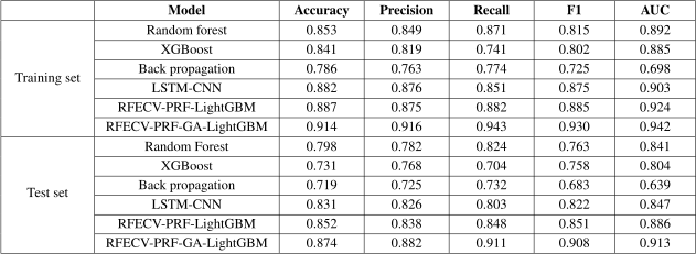
To validate the scalability of the model, data samples from the CSMAR and Resset databases, covering financial and non-financial data from 2008 to 2022, were used. The dataset includes 39,356 observations, excluding companies in the financial sector 29.
Building on a systematic review of corporate financial fraud research, this study constructs a multi-dimensional fraud detection framework based on the CSMAR and Resset dual-source databases, taking into account differences in indicator attributes. The framework divides the analysis dimensions into two main categories: financial and non-financial. The financial dimension focuses on three core areas: corporate solvency (current ratio, quick ratio), asset operating efficiency (inventory turnover, total asset turnover), and profitability quality (leverage ratio, return on total assets, return on equity). These parameters directly reflect the company’s financial condition and operational effectiveness. The non-financial dimension incorporates structural variables such as corporate nature (company type), governance characteristics (dual roles, size of the supervisory board), market relationships (shareholding ratio of institutional investors, audit firm type), and strategic elements (political connections, company size, R&D investment ratio). These factors reveal how organizational decision-making mechanisms have a substantial impact on fraud risk.
The performance of each model in identifying financial fraud is shown in Table 11.
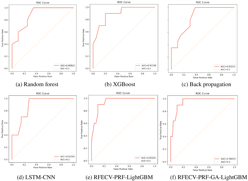
Fig. 4. ROC curves of different models.
Table 11. Performance of different models on public datasets.
4. Conclusion
This study proposes a novel solution to the problem of corporate financial fraud detection by constructing a model based on RFECV-PRF feature selection and GA-LightGBM optimization. The results indicate that this model outperforms traditional methods across multiple industry datasets, particularly in key metrics such as accuracy, recall, and F1 score. By combining RFECV and PRF, the model effectively eliminates redundant features, reducing computational complexity while improving the precision of data analysis. The optimization of LightGBM parameters using GA further enhances the model’s adaptability and robustness in complex data environments.
In practical applications, this model serves as an efficient intelligent tool, helping businesses and regulatory bodies quickly identify financial fraud, thereby reducing investment risks and maintaining market order. Future research could focus on further optimizing the model’s complexity and operational efficiency to meet the real-time analysis needs of larger-scale datasets.
- [1] S. Cai, “Explainable fraud detection of financial statement data driven by two-layer knowledge graph,” Expert Syst. Appl., Vol.246, Article No.123126, 2024. https://doi.org/10.1016/j.eswa.2023.123126
- [2] W. Zhou, “Detecting evolutionary financial statement fraud,” Decis. Support Syst., Vol.50, No.3, pp. 570-575, 2011. https://doi.org/10.1016/j.dss.2010.08.007
- [3] D. Kong, “Explain or conceal? Causal language intensity in annual report and stock price crash risk,” Econ. Model., Vol.94, pp. 715-725, 2021. https://doi.org/10.1016/j.econmod.2020.02.013
- [4] J. Li, “Textual analysis and detection of financial fraud: Evidence from Chinese manufacturing firms,” Econ. Model., Vol.126, Article No.106428, 2023. https://doi.org/10.1016/j.econmod.2023.106428
- [5] Y. Li, B. Fu, Y. Tong, Z. Tang, Z. Shang, and A. Li, “Abnormal detection of financial fraud in listed companies based on deep learning,” Procedia Comput. Sci., Vol.242, pp. 1402-1409, 2024. https://doi.org/10.1016/j.procs.2024.08.112
- [6] K. G. Al-Hashedi and P. Magalingam, “Financial fraud detection applying data mining techniques: A comprehensive review from 2009 to 2019,” Comput. Sci. Rev., Vol.40, Article No.100402, 2021. https://doi.org/10.1016/j.cosrev.2021.100402
- [7] J. West, “Intelligent financial fraud detection: A comprehensive review,” Computers & Security, Vol.57, pp. 47-66, 2016. https://doi.org/10.1016/j.cose.2015.09.005
- [8] T. Prabhavathy, V. K. Elumalai, and E. Balaji, “Hand gesture classification framework leveraging the entropy features from sEMG signals and VMD augmented multi-class SVM,” Expert Syst. Appl., Vol.238, Part D, Article No.121972, 2024. https://doi.org/10.1016/j.eswa.2023.121972
- [9] G. G. Sundarkumar, V. Ravi, and V. Siddeshwar, “One-class support vector machine based undersampling: Application to churn prediction and insurance fraud detection,” 2015 IEEE Int. Conf. on Computational Intelligence and Computing Research (ICCIC), 2015. https://doi.org/10.1109/ICCIC.2015.7435726
- [10] Q. Deng, “Application of support vector machine in the detection of fraudulent financial statements,” 2009 4th Int. Conf. on Computer Science & Education, pp. 1056-1059, 2009. https://doi.org/10.1109/ICCSE.2009.5228542
- [11] H. Pan, “Incremental model checking for fuzzy computation tree logic,” Fuzzy Sets Syst., Vol.500, Article No.109195, 2025. https://doi.org/10.1016/j.fss.2024.109195
- [12] K. Supraja and S. J. Saritha, “Robust fuzzy rule based technique to detect frauds in vehicle insurance,” 2017 Int. Conf. on Energy, Communication, Data Analytics and Soft Computing (ICECDS), pp. 3734-3739, 2017. https://doi.org/10.1109/ICECDS.2017.8390160
- [13] S. K. Saeed and H. Hagras, “Adaptive type-2 fuzzy logic based system for fraud detection in financial applications,” 2018 10th Computer Science and Electronic Engineering (CEEC), pp. 15-18, 2018. https://doi.org/10.1109/CEEC.2018.8674217
- [14] S. Z. Aftabi, A. Ahmadi, and S. Farzi, “Fraud detection in financial statements using data mining and GAN models,” Expert Syst. Appl., Vol.227, Article No.120144, 2023. https://doi.org/10.1016/j.eswa.2023.120144
- [15] I. Dutta, S. Dutta, and B. Raahemi, “Detecting financial restatements using data mining techniques,” Expert Syst. Appl., Vol.90, pp. 374-393, 2017. https://doi.org/10.1016/j.eswa.2017.08.030
- [16] P. Hajek, “Interpretable fuzzy rule-based systems for detecting financial statement fraud,” J. MacIntyre, I. Maglogiannis, L. Iliadis, and E. Pimenidis (Eds.), “Artificial intelligence applications and innovations,” Springer, pp. 425-436, 2019. https://doi.org/10.1007/978-3-030-19823-7_36
- [17] M. Lokanan, V. Tran, and N. H. Vuong, “Detecting anomalies in financial statements using machine learning algorithm: The case of Vietnamese listed firms,” Asian J. Account. Res., Vol.4, No.2, pp. 181-201, 2019. https://doi.org/10.1108/AJAR-09-2018-0032
- [18] Indrajani, Y. Heryadi, L. A. Wulandhari, and B. S. Abbas, “Recognizing debit card fraud transaction using CHAID and K-nearest neighbor: Indonesian Bank case,” 2016 11th Int. Conf. on Knowledge, Information and Creativity Support Systems (KICSS), 2016. https://doi.org/10.1109/KICSS.2016.7951441
- [19] V. R. Sonwane, S. Zanje, S. Yenpure, Y. Gunjal, Y. Kulkarni, and R. Yeole, “Advanced machine learning techniques for credit card fraud detection: A comprehensive study,” 2024 5th Int. Conf. on Smart Electronics and Communication (ICOSEC), pp. 1978-1981, 2024. https://doi.org/10.1109/ICOSEC61587.2024.10722667
- [20] U. Jabeen, K. Singh, and S. Vats, “Credit card fraud detection scheme using machine learning and synthetic minority oversampling technique (SMOTE),” 2023 5th Int. Conf. on Inventive Research in Computing Applications (ICIRCA), pp. 122-127, 2023. https://doi.org/10.1109/ICIRCA57980.2023.10220646
- [21] A. Singh, A. Singh, A. Aggarwal, and A. Chauhan, “Design and implementation of different machine learning algorithms for credit card fraud detection,” 2022 Int. Conf. on Electrical, Computer, Communications and Mechatronics Engineering (ICECCME), 2022. https://doi.org/10.1109/ICECCME55909.2022.9988588
- [22] P. Hajek and R. Henriques, “Mining corporate annual reports for intelligent detection of financial statement fraud – A comparative study of machine learning methods,” Knowl.-Based Syst., Vol.128, pp. 139-152, 2017. https://doi.org/10.1016/j.knosys.2017.05.001
- [23] T. Shahana, “State of the art in financial statement fraud detection: A systematic review,” Technol. Forecast., Vol.192, Article No.122527, 2023. https://doi.org/10.1016/j.techfore.2023.122527
- [24] Y. Zhang, A. Hu, J. Wang, and Y. Zhang, “Detection of fraud statement based on word vector: Evidence from financial companies in China,” Finance Res. Lett., Vol.46, Article No.102477, 2022. https://doi.org/10.1016/j.frl.2021.102477
- [25] S. A. Naghibi, H. Hashemi, R. Berndtsson, and S. Lee, “Application of extreme gradient boosting and parallel random forest algorithms for assessing groundwater spring potential using DEM-derived factors,” J. Hydrol., Vol.589, Article No.125197, 2020. https://doi.org/10.1016/j.jhydrol.2020.125197
- [26] A. Habibi, M. R. Delavar, M. S. Sadeghian, B. Nazari, and S. Pirasteh, “A hybrid of ensemble machine learning models with RFE and Boruta wrapper-based algorithms for flash flood susceptibility assessment,” Int. J. Appl. Earth Obs. Geoinformation, Vol.122, Article No.103401, 2023. https://doi.org/10.1016/j.jag.2023.103401
- [27] F. Li, “Network traffic prediction based on PSO-LightGBM-TM,” Comput. Netw., Vol.254, Article No.110810, 2024. https://doi.org/10.1016/j.comnet.2024.110810
- [28] F. Jiang et al., “Thermal performance prediction of radial-rotating oscillating heat pipe by a novel fusion model: A case study of application in grinding,” Case Stud. Therm. Eng., Vol.60, Article No.104731, 2024. https://doi.org/10.1016/j.csite.2024.104731
- [29] X. Yuan, Y. Zhou, C. Yan, Y. Wang, H. He, and Q. Zhang, “Extraction of features for financial fraud in companies using machine learning algorithms,” SmartTech Innov., Vol.1, No.1, pp. 28-38, 2025. https://doi.org/10.26917/j.cnki.issn.2097-597X.2025.01.003
This article is published under a Creative Commons Attribution-NoDerivatives 4.0 Internationa License.