Research Paper:
Unknown Input Observer Designs for Polynomial Fuzzy Systems with Uncertainties
Xiang Wang
 , Lizhen Li†
, and Yutang Wu
, Lizhen Li†
, and Yutang Wu
College of Mathematics and Physics, Shanghai University of Electric Power
No.1851 Hucheng Ring Road, Pudong New Area, Shanghai 201306, China
†Corresponding author

This study developed a novel design framework for unknown input observers in uncertain polynomial fuzzy systems using the sum-of-squares algorithm. First, both the system and the input matrices depended on unmeasurable state variables that required estimation. Secondly, the observer structure in this study differed from existing formulations. The proposed observer eliminated uncertainty effects without requiring explicit bounds or auxiliary controllers. The incorporation of slack matrices facilitated the resolution of non-convex terms in the stability conditions, thereby reducing design conservatism. Finally, a simulation study was conducted, and the results confirmed the validity and theoretical value of the developed strategy.
Errors converge globally
1. Introduction
The Takagi–Sugeno (T–S) fuzzy framework 1,2 was proposed in 1985, providing a landmark contribution that paved the way for systematic studies of nonlinear systems. This model has attracted significant attention in control system researches. Subsequently, numerous theories and designs of nonlinear control systems built on the T–S framework have emerged. Illustrative examples include observer-based switching controllers for fuzzy plants with mixed time delays 3. At a broader level, a novel fuzzy Lyapunov function for continuous-time control systems was introduced 4.
Recent advances have established polynomial fuzzy systems (PFSs) as powerful extensions of the T–S model, leveraging polynomial Lyapunov functions and sum-of-squares (SOS) techniques 5,6. Extensive research has focused on PFSs, including controller designs, observer designs, and stability analysis 7,8,9,10,11,12,13,14. For example, 7 used switching polynomial Lyapunov functions comprising of multiple local Lyapunov functions to investigate stabilization, achieving more relaxed stability conditions. Furthermore, unknown input observer designs for PFSs based on the SOS algorithm were investigated in 15.
As evidenced by the literature, polynomial observer designs have received increasing attention. However, technical limitations and economic constraints often prevent the measurement of certain state variables that are indispensable for both observer and controller designs in nonlinear systems. To address this challenge, several approaches have been developed in recent years for PFSs with partially or completely unmeasurable state variables 16,17,18,19. Seo et al. 16 and Tanaka et al. 17 addressed the stabilization of nonlinear control systems and guaranteed the asymptotic convergence of state estimation errors to zero. This was achieved using polynomial fuzzy observers that leveraged the separation principle. Building upon this work, the SOS-based framework was further generalized to discrete-time cases in subsequent researches 18,19.
In practical applications, numerous systems are subject to uncertainties. These uncertainties significantly complicate the design of observers and controllers for these systems. Prior studies addressed uncertainty problems based on the T–S fuzzy model 20,21,22,23,24,25,26. Additionally, robust control of PFSs with uncertainties was investigated using the SOS algorithm 27,28, and observer designs for PFSs with unknown inputs were explored 29,30.
Whereas most existing observer designs assume that polynomial system matrices depend solely on measurable state variables 17, few studies address scenarios in which matrices depend on unmeasurable state variables that require estimation. Extending the work in 21,28, we developed an observer framework in which polynomial system and input matrices depended on unmeasurable state variables. All the design conditions were formulated and solved using SOSTOOLS in MATLAB. The proposed design methodology for PFSs with uncertainties has significant potential for applications in various complex nonlinear systems. Furthermore, the robustness analysis for unbounded uncertainties suggests its applicability in aerospace systems, such as aircraft attitude control and hypersonic vehicle dynamics, in which modeling uncertainties and disturbance rejection are critical concerns.
Building on the existing literature, this study makes the following primary contributions:
-
(1)
This study developed an unknown input observer framework for PFSs with uncertainties. Crucially, both polynomial system and input matrices could depend on unmeasurable state variables that require estimation, representing a significant departure from conventional designs that are limited to measurable state variables. The proposed observer eliminated uncertainty effects without requiring explicit bounds or auxiliary controllers.
-
(2)
This study derived the SOS stability conditions using polynomial fuzzy Lyapunov functions that incorporated unmeasurable state variables. By employing slack matrices, the nonconvex terms in the stability conditions were resolved, thereby reducing design conservatism.
To ensure consistency, we adopt the following notation: \(A > 0\) denotes a positive definite matrix. The transpose and inverse of \(A\) are represented as \(A^T\) and \(A^{-1}\), respectively. For a matrix \(A\) with full column rank, its Moore–Penrose pseudoinverse, denoted \(A^†\), is computed as \(A^†=(A^T A)^{-1}A^T\). \(I\) signifies the identity matrix, and symbol \(\ast\) is used within symmetric matrices to indicate the transposed elements.
2. Polynomial Fuzzy System Representation
Consider the following nonlinear system.
Here, the dynamics of nonlinear system contain possible uncertainties, \(z(t) \in \Re^{n}\) represents the unmeasurable state variable, \(u(t) \in \Re^{m}\) represents the controlled input, and \(\upsilon(t)\) represents the vector of time-varying parameters. \(C\) represents an output matrix whose entries are all constants, and \(y(t)\) represents the measurable output vector of the system. By applying the sector nonlinearity approach, we obtain a representation of the nonlinear system using \(r\) fuzzy rules. Plant Rule \(i\): if \(\phi_1(z(t))\) \(\textrm{is}\) \(Z_1^i\), \(\phi_2(z(t))\) \(\textrm{is}\) \(Z_2^i,\ldots ,\phi_s(z(t))\) \(\textrm{is}\) \(Z_s^i\), then
The fuzzy rule structure employs premise variables \(\phi_l(z(t))\), with \(Z_l^i\) being the associated membership function for the \(i\)-th rule. The dynamics of a nonlinear system are parameterized by known matrices \(A_i(z(t)) \in \Re^{n \times N}\) and \(B_i(z(t)) \in \Re^{n \times m}\), along with their uncertainties \(\Delta A_i(z(t)) \in \Re^{n \times N}\) and \(\Delta B_i(z(t)) \in \Re^{n \times m}\). Nonlinear plant (Eq. (2)) explicitly maintains the dependence on unmeasurable state variables while accounting for unbounded uncertainties in the system dynamics.
The global dynamics of the uncertain PFS derived through the weighted aggregation of the plant rules in Eq. (2) can be expressed as follows:
All the matrices in PFS (Eq. (3)) depend on the state variables, creating fundamental challenges for observer design. Notably, the polynomial and uncertainty matrices are both parameterized by unmeasurable state \(z(t)\) that must be estimated. This dependency creates a complex theoretically estimation problem.
However, prior research 17 addressed systems with state-dependent matrices involving unmeasurable state variables. The existing approaches in this study suffer from two drawbacks: they require simultaneous observer controller design and depend on known uncertainty bounds. We developed an SOS-based observer that handles state-dependent matrices and unbounded uncertainties. Simultaneously, to mitigate the conservatism inherent in the stability analysis and handle the complexity of the system, slack matrices were strategically introduced. This technique relaxed the original stringent stability conditions, thereby transforming them into a collection of conditions that were more manageable and amenable to numerical solutions via convex optimization.
For notational conciseness, the time argument \(t\) is dropped hereafter. Simplified notations \(z\) and \(\hat{z}\) represent \(z(t)\) and \(\hat{z}(t)\), respectively, where \(\hat{z}(t)\) represents the estimation of real state \(z(t)\). When adopting this simplified notation, all variables remain time-dependent quantities in the system dynamics.
3. Theoretical Analysis of Observer Synthesis
Prior to the theoretical derivation, the following assumptions must first be established.
Assumption 1: The system uncertainties admit the following equations.
Assumption 2: Output matrix \(C\) has full row rank. Rank conditions \(\text{rank}(CD_A(z))=\text{rank}(D_A(z))\) and \(\text{rank}(CD_B(z))=\text{rank}(D_B(z))\) hold for state variable \(z\).
Remark 1: Assumption 1 enables the transformation of system uncertainties into unknown input terms, whereas Assumption 2 ensures that the matrix equation admits a general solution, the specific form of which is presented in Theorem 2.
Under Assumption 1, uncertain PFS (Eq. (3)) is transformed into an unknown input PFS. We define the equivalent unknown inputs, \(\gamma_i=\Delta\widetilde{A}_i(z)z\) and \(\sigma_i=\Delta\widetilde{B}_i(z)u\), both of which are vectors in \(\Re^q\). The fuzzy model can be expressed as follows:
Defining \(\omega_i=\gamma_i+\sigma_i\), we obtain the dynamics of nonlinear system representation as follows:
This leads to the following observer.
From Eq. (5), we can obtain the following.
The error state is defined as \(e = z - \hat{z}\). Consequently, the dynamics are given by
Substituting PFS (Eq. (5)) and observer (Eq. (6)) into error dynamics (Eq. (8)), we obtain the following:
By substituting output derivative expression (Eq. (7)) into error dynamics (Eq. (9)), we obtain the complete error dynamics representation.
We now introduce an assumption on the membership functions for proving Theorem 1.
Assumption 3: Known positive constants \(\theta_k > 0\) exist such that \(|\dot{\beta}_k(\upsilon)| \leq \theta_k\), for \(k=1,2,\dots,r\).
Theorem 1: Consider PFS (Eq. (5)) under the aforementioned assumptions. Achieving asymptotic convergence of the estimation error in observer (Eq. (6)) is contingent on the existence of polynomial matrices \(F(z)\), \(N_i(z,\hat{z})\), \(L_i(\hat{z})\), and \(G_i(z)\) and symmetric positive definite matrices \(P_i\) that fulfill the following.
Proof: Upon satisfying conditions (11)–(13) in Theorem 1, error dynamics (Eq. (10)) is simplified to
Consider the following fuzzy Lyapunov function candidate.
It follows directly from condition (14) that each Lyapunov matrix \(P_i\) is symmetric and positive definite, characterized by \(P_i=P_i^T>0\).
Under Eq. (17) and Assumption 3, we compute the derivative of the Lyapunov function with respect to time as follows:
From inequality (18), the satisfaction of condition (15) directly ensures that \(\dot{V}<0\); this proves \(e\rightarrow0\) as \(t\rightarrow\infty\), thereby completing the proof of Theorem 1. For observer synthesis, the matrices \(N_i(z,\hat{z})\), \(G_i(z)\), \(L_i(\hat{z})\), and \(F(z)\) must satisfy conditions (11)–(15). However, the presence of bilinear terms in condition (15) presents a computational challenge. Next, we must transform these into convex terms that can be solved by using SOSTOOLS in MATLAB.
Lemma 1: Let \(M^+=(M^TM)^{-1}M^T\) be the Moore–Penrose pseudoinverse of \(M\in\Re^{m\times n}\). For \(W\in\Re^{k\times n}\), condition \(WM^+M=W\) is necessary and sufficient for the existence of solutions to \(HM=W\). Under this condition, the general solution is \(H=WM^++Y(I-MM^+)\), where \(Y\in\Re^{k\times m}\) is an arbitrary matrix.
Lemma 2: For matrices \(A\), \(S\), \(P\), and \(R\) with compatible dimensions, the following conditions are equivalent.
Theorem 2: Under the aforementioned assumptions, the estimation error \(e\) of observer (Eq. (6)) asymptotically converges to zero if polynomial matrices \(F(z)\), \(N_i(z,\hat{z})\), \(L_i(\hat{z})\), \(G_i(z)\), \(K(z)\), \(X(z)\), and \(Q(z,\hat{z})\) exist and symmetric positive definite matrices \(P_i\) satisfy the following conditions.
Proof: The following auxiliary matrices are defined.
Furthermore, the polynomial matrices in Eq. (6) are explicitly given by
From condition (15) of Theorem 1, we directly obtain the following matrix inequality.
By applying Lemma 2 to inequality (32) by introducing slack variable \(X(z)\), we obtain the following equivalent matrix inequality.
From condition (13), we directly the following equation.
Applying Lemma 1 to Eq. (36), the general solution is expressed as follows:
Under Assumption 2, which applies to matrices \(C\) and \(D(z)\), a general solution (Eq. (38)) exists.
We define the following auxiliary matrices.
Substituting Eqs. (39) and (40) into Eq. (37) yields the following polynomial matrix.
Combining Eqs. (11) and (41), we derive the following polynomial matrix.
Substituting Eq. (42) into Eq. (34) yields the explicit matrix expression for \(\Phi_{ik}^{11}\).
Substituting Eq. (42) into Eq. (35) yields the complete expression for \(\Omega_{ij}^{21}\).
To facilitate subsequent derivations, we introduce the following auxiliary matrices.
By applying auxiliary matrices (Eqs. (45) and (46)), we derive the final matrix forms as follows:
Combining expressions (47) and (48), we transform inequality (33) into the following equivalent form.
Note that Eq. (49) is algebraically equivalent to condition (20) in Theorem 2. This demonstrates that the originally non-convex terms in Eq. (15) have been transformed into convex terms that are directly solvable using SOSTOOLS in MATLAB.
4. Example of Numerical Simulation
The validity and theoretical value of the proposed SOS-based design for synthesizing observers for uncertain PFSs are established by the numerical simulation presented as follows:
Consider the control system represented by the following formulation:
The membership derivatives satisfy: \(|\dot{\beta}_1(\upsilon)| = |\mbox{$-\dot{z}_2({\sin(z_2)}/{2})$}|\), \(|\dot{\beta}_2(\upsilon)| = |\dot{z}_2({\sin(z_2)}/{2})|\). Consistent with Assumption 3, we set \(\theta_1=\theta_2=0.4\).
Consider that system (52) is subject to unbounded uncertainties, and the bounded constraints are unknown. This can be represented as follows:
System (53) is transformed into a system with unknown inputs. This transformation yields the following.
We select
Step \(1\): Both \(C\) and \(D(z)\) have full rank, with \(\text{rank}(CD(z))=\text{rank}(D(z))=1\), thereby fulfilling Assumption 2.
Step \(2\): Applying definitions (39) and (40) yields the following:
Step \(3\): Solving SOS conditions (Eqs. (19) and (20)) using SOSTOOLS in MATLAB yields the following.
Step \(4\): Observer matrices \(F(z)\), \(G_i(z)\), \(L_i(\hat{z})\), and \(N_i(z,\hat{z})\) are solved using Eqs. (28)–(31).
Under the following simulation setup, the input used for the simulation was \(u=0.2\sin(t)\), and the parameters were \(\delta_1(z,\hat{z})=\delta_2(z,\hat{z})=10^{-9}\).
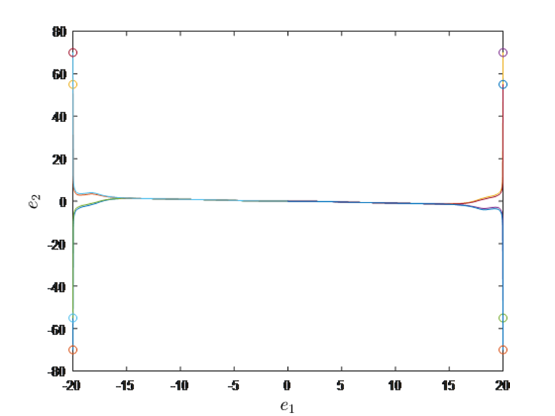
Figure 1 presents estimation errors \(e_1\) and \(e_2\) for ten distinct initial errors. Phase portrait analysis demonstrated asymptotic convergence from diverse initial errors, validating the global stability of the observer. Under the initial states, \(z(0) = [-100\hspace{1em} -150]^T\) and \(\hat{z}(0) = [-80\hspace{1em} -215]^T\), the state evolution of the system was recorded. The results for the real and estimated states are shown in Figs. 2 and 3, respectively. Figs. 4 and 5 depict the time responses of estimation errors \(e_1\) and \(e_2\), respectively, under initial error \(e(0)=[-20\hspace{1em}65]^T\). The figures exhibit the asymptotical convergence of the estimation errors to zero.
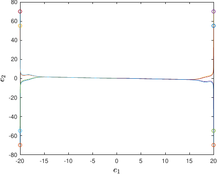
Fig. 1. Estimation errors \(e_1\) and \(e_2\).
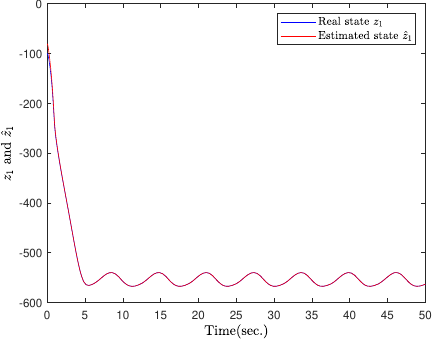
Fig. 2. Time responses for the \(z_1\) and \(\hat{z}_1\).
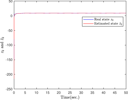
Fig. 3. Time responses for the \(z_2\) and \(\hat{z}_2\).
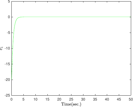
Fig. 4. Estimation error \(e_1\).
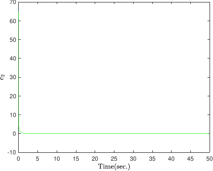
Fig. 5. Estimation error \(e_2\).
Table 1. Performance comparison between the proposed method and 8,17.

In addition, we compared the performance of our method with those of 8,17. As summarized in Table 1, the root mean square error (RMSE) is defined as \(\textit{RMSE}=\sqrt{({1}/{N})\sum^{N}_{p=1}\|e(p)\|^2}\). \(N\), indicating the number of samples, and convergence time \(t_s\), measured as the time required for the estimation errors to reach a threshold \(1\times10^{-4}\), were evaluated. The quantitative results demonstrated that the proposed method outperformed existing approaches 8,17 in terms of both convergence speed and robustness. These findings conclusively validated the proposed observer synthesis methodology for uncertain PFSs.
5. Conclusion
This paper presents an unknown input observer design for uncertain PFSs using the SOS algorithm. Two theorems were developed to support the observer synthesis framework. The resulting convex conditions were solvable using SOSTOOLS in MATLAB. The core contributions included the following. First, a novel polynomial observer was developed that was distinct from existing formulations. Crucially, both the system and input matrices could be dependent on the unmeasurable state variable. Second, uncertainty effects were eliminated without requiring explicit bounds. Third, the nonconvex terms in the stability conditions were resolved through slack matrices in Theorem 2, thus reducing design conservatism. Finally, a numerical validation confirmed the theoretical value of the proposed methodology for uncertain PFSs.
Acknowledgments
This research was supported by the National Natural Science Foundation of China under Grant No.61903244.
- [1] T. Takagi and M. Sugeno, “Fuzzy identification of systems and its applications to modeling and control,” IEEE Trans. on Syst. Man Cybern., Vol.15, No.1, pp. 116-132, 1985. https://doi.org/10.1109/TSMC.1985.6313399
- [2] M. Sugeno and G. T. Kang, “Structure identification of fuzzy model,” Fuzzy Sets Syst., Vol.28, No.1, pp. 15-33, 1988. https://doi.org/10.1016/0165-0114(88)90113-3
- [3] M. Xu, J. Gu, and Z. Xu, “Observer-based switching control for T–S fuzzy systems with mixed time delays,” Int. J. of Fuzzy Systems, Vol.25, No.4, pp. 1480-1494, 2023. https://doi.org/10.1007/s40815-022-01447-0
- [4] B. J. Rhee and S. Won, “A new fuzzy Lyapunov function approach for a Takagi–Sugeno fuzzy control system design,” Fuzzy Sets Syst., Vol.157, No.9, pp. 1211-1228, 2006. https://doi.org/10.1016/j.fss.2005.12.020
- [5] K. Tanaka, H. Yoshida, and H. Ohtake, “A sum-of-squares approach to modeling and control of nonlinear dynamical systems with polynomial fuzzy systems,” IEEE Trans. on Fuzzy Syst., Vol.17, No.4, pp. 911-922, 2009. https://doi.org/10.1109/TFUZZ.2008.924341
- [6] K. Tanaka, H. Ohtake, and H. O. Wang, “Guaranteed cost control of polynomial fuzzy systems via a sum of squares approach,” IEEE Trans. on Syst. Man Cybern., Vol.39, No.2, pp. 561-567, 2009. https://doi.org/10.1109/TSMCB.2008.2006639
- [7] H. K. Lam, M. Narimani, and H. Li, “Stability analysis of polynomial-fuzzy-model-based control systems using switching polynomial Lyapunov function,” IEEE Trans. on Fuzzy Syst., Vol.21, No.5, pp. 800-813, 2013. https://doi.org/10.1109/TFUZZ.2012.2230005
- [8] K. Y. Ye, J. Li, and Y. G. Niu. “Disturbance-observer-based sliding mode control for polynomial fuzzy systems,” Int. J. of Systems Science, pp. 1-5, 2025. https://doi.org/10.1080/00207721.2025.2491780
- [9] B. Pang and Q. Zhang, “Interval observers design for polynomial fuzzy singular systems by utilizing sum-of-squares program,” IEEE Trans. Systs., Man, Cybern., Syst., Vol.50, No.6, pp. 1999-2006, 2020. https://doi.org/10.1109/TSMC.2018.2790975
- [10] D. Pylorof, E. Bakolas, and K. S. Chan, “Design of robust Lyapunov-based observers for nonlinear systems with sum-of-squares programming,” IEEE Control Syst. Letters, Vol.4, No.2, pp. 283-288, 2019. https://doi.org/10.1109/LCSYS.2019.2925511
- [11] H. Han, Y. Sueyama, and C. Chen, “A design of observers of control state and uncertainty via transformation of T-S fuzzy models,” J. Adv. Comput. Intell. Intell. Inform., Vol.22, No.2, pp. 194-202, 2018. https://doi.org/10.20965/jaciii.2018.p0194
- [12] F. Sabbaghian and M. Farrokhi, “Polynomial fuzzy observer-based integrated fault estimation and fault tolerant control with uncertainty and disturbance,” IEEE Trans. Fuzzy Syst., Vol.30, No.3, pp. 741-754, 2020. https://doi.org/10.1109/TFUZZ.2020.3048505
- [13] X. Wang, L. Li, and Y. Wu, “Static output feedback controller design for switching polynomial fuzzy time-varying delay system,” J. Adv. Comput. Intell. Intell. Inform., Vol.28, No.6, pp. 1335-1343, 2024. https://doi.org/10.20965/jaciii.2024.p1335
- [14] V. P. Vu and W. J. Wang, “State and disturbance observer-based controller synthesis for polynomial system,” 2017 Int. Conf. on System Science and Engineering (ICSSE), pp. 66-70, 2017. https://doi.org/10.1109/ICSSE.2017.8030839
- [15] V. P. Vu, W. J. Wang, H. C. Chen, and J. M. Zurada, “Unknown input-based observer synthesis for a polynomial T-S fuzzy model system with uncertainties,” IEEE Trans. Fuzzy Syst., Vol.26, No.3, pp. 1447-1458, 2018. https://doi.org/10.1109/TFUZZ.2017.2724507
- [16] T. Seo, H. Ohtake, K. Tanaka, Y. J. Chen, and H. O. Wang, “A polynomial observer design for a wider class of polynomial fuzzy systems,” 2011 IEEE Int. Conf. on Fuzzy Systems, pp. 1305-1311, 2011. https://doi.org/10.1109/FUZZY.2011.6007342
- [17] K. Tanaka, H. Ohtake, and T. Seo, “Polynomial fuzzy observer designs: A sum-of-squares approach,” IEEE Trans. Syst. Man Cybern. Part B, Vol.42, No.5, pp. 1330-1342, 2012. https://doi.org/10.1109/TSMCB.2012.2190277
- [18] N. Azman, S. Saat, and S. K. Nguang, “Nonlinear observer design with integrator for a class of polynomial discrete-time systems,” 2015 Int. Conf. on Computer, Communications, and Control Technology, pp. 422-426, 2015. https://doi.org/ 10.1109/I4CT.2015.7219611
- [19] Y. Wang, H. Zhang, and J. Zhang, “An SOS-based observer design for discrete-time polynomial fuzzy systems,” Int. J. of Fuzzy Syst., Vol.17, No.1, pp. 94-104, 2015. https://doi.org/10.1007/s40815-015-0003-x
- [20] J. Zhao and H. Han, “A control approach based on observers of state and uncertainty for a class of Takagi–Sugeno fuzzy models,” J. Adv. Comput. Intell. Intell. Inform., Vol.25, No.3, pp. 317-325, 2021. https://doi.org/10.20965/jaciii.2021.p0317
- [21] W. J. Wang, V. P. Vu, and W. Chang, “A synthesis of observer-based controller for stabilizing uncertain T-S fuzzy systems,” J. of Intell. Fuzzy Syst., Vol.30, No.6, pp. 3451-3463. https://doi.org/10.1049/iet-cta.2017.0489
- [22] A. Golabi, M. Beheshti, and M. Asemani, “ H_infty H∞ robust fuzzy dynamic observer-based controller for uncertain Takagi–Sugeno fuzzy systems,” IET Control Theory and Applications, Vol.6, No.10, pp. 1434-1444, 2011 https://doi.org/10.1049/iet-cta.2011.0435
- [23] T. Dang, W. J. Wang, and C. H. Huang, “Observer synthesis for the T-S fuzzy system with uncertainty and output disturbance,” J. of Intell. Fuzzy Syst., Vol.22, No.4, pp. 173-183, 2011. https://doi.org/10.3233/IFS-2011-0474
- [24] V. P. Vu and W. J. Wang, “Observer synthesis for uncertain Takagi–Sugeno fuzzy systems with multiple output matrices,” IET Control Theory and Applications, Vol.10, No.2, pp. 151-161, 2016. https://doi.org/10.1049/iet-cta.2015.0228
- [25] J. S. Yeh, W. Chang, and W. J. Wang, “Unknown input based observer synthesis for uncertain Takagi–Sugeno fuzzy systems,” IET Control Theory and Applications, Vol.9, No.5, pp. 729-735, 2015. https://doi.org/10.1049/iet-cta.2014.0705
- [26] V. P. Vu and W. J. Wang, “Observer design for a discrete-time T-S fuzzy system with uncertainties,” 2015 IEEE Int. Conf. on Automation Science and Engineering, pp. 1262-1267, 2015. https://doi.org/10.1109/CoASE.2015.7294272
- [27] H. S. Kim, J. B. Park, and Y. H. Joo, “Robust stabilization condition for a polynomial fuzzy system with parametric uncertainties,” 2012 12th Int. Conf. on Control, Automation and Systems, pp. 107-111, 2012.
- [28] K. Tanaka, M. Tanaka, Y. J. Chen, and H. O. Wang, “A new sum-of-squares design framework for robust control of polynomial fuzzy systems with uncertainties,” IEEE Trans. Fuzzy Systs., Vol.24, No.1, pp. 94-110, 2016. https://doi.org/10.1109/TFUZZ.2015.2426719
- [29] A. Chibani, M. Chadli, M. M. Belhaouane, and N. B. Braiek, “Polynomial observer design for unknown inputs polynomial fuzzy systems: A sum of squares approach,” IEEE Conf. on Decision and Control, pp. 6788-6793, 2015. https://doi.org/10.1109/CDC.2014.7040455
- [30] A. Chibani, M. Chadli, and N. B. Braiek, “A sum of squares approach for polynomial fuzzy observer design for polynomial fuzzy systems with unknown inputs,” Int. J. of Control Auto. and Syst., Vol.14, No.1, pp. 323-330, 2016. https://doi.org/10.1007/s12555-014-0406-8
This article is published under a Creative Commons Attribution-NoDerivatives 4.0 Internationa License.