Research Paper:
Emotion Analysis in the Human Brain Evoked by Language Stimulation
Eri Miura
 and Ichiro Kobayashi
Ochanomizu University
2-1-1 Ohtsuka, Bunkyo-ku, Tokyo 112-8610, Japan

Advances in neural recording and deep learning have enabled a more precise analysis of how the brain processes language. However, neural representations of diverse emotions during natural narrative language comprehension remains unclear. In this study, we investigated how emotional content in naturalistic spoken language is reflected in brain activity using two independent narrative functional magnetic resonance imaging datasets: Alice and Le Petit Prince. Participants listened to narrative readings and their blood-oxygenation-level-dependent responses were recorded. An emotion recognition model was developed by fine-tuning BERT using the GoEmotions dataset together with sentence-level annotations for 80 emotions. Emotional and linguistic features were extracted and used to train voxel-wise encoding models to predict brain activity. To examine emotion-related neural representations, we subtracted predictions based on linguistic features from those based on combined emotional and linguistic features. The resulting emotion-related activity patterns were distributed across cortical regions associated with affective and semantic processing and were consistent across subjects and datasets. These findings indicate that the emotional meaning conveyed through natural language is represented in a graded and distributed manner in the human brain, beyond linguistic content alone.
Extracting linguistic and emotional features using BERT to predict brain activity
1. Introduction
In recent years, research has focused on analyzing brain activity data obtained from functional magnetic resonance imaging (fMRI) and predicting brain activity using data-driven approaches 1. However, much remains unknown about how emotions are represented in the human brain. This study investigates emotional responses in the human brain under linguistic stimuli. Specifically, we predict emotion-related brain activity using fMRI data recorded from subjects who listened to narrative readings, together with the linguistic and emotional features extracted from each sentence.
2. Related Work
Table 1. Eighty emotion categories.

Recent years have seen a surge in behavioral studies that use large-scale data to reveal the complex structure of human emotions. Cowen et al. 2,3,4 demonstrated that a wide range of emotional experiences can be evoked by diverse types of stimuli, such as videos, sounds, and facial expressions. These findings suggest that emotions can be represented in a high-dimensional space, motivating efforts to explore how such emotional structures are reflected in brain activity. In neuroscience, one powerful approach is the use of continuous semantic spaces and voxel-wise encoding models 1,5,6, which examine how different concepts and emotional categories are organized across the cortex. Building on this approach, Koide-Majima et al. 7 used fMRI data collected during video viewing to show how 80 emotion categories were mapped onto the brain surface. More recently, Wallenwein et al. 8 demonstrated that the brain encodes emotional expressions consistently across different sensory inputs, such as voices and faces, suggesting that emotions are represented in a shared, cross-modal format. Batten et al. 9 provided direct evidence of how emotional words affect brain chemistry. By simultaneously measuring dopamine, serotonin, and norepinephrine release in the human brain, they found that different emotions trigger specific neurochemical responses in regions such as the thalamus and anterior cingulate cortex. However, most of these studies focused on visual or facial stimuli, and it remains unclear how the brain represents emotions conveyed through natural language. In this study, we addressed this gap by analyzing fMRI responses recorded while participants listened to spoken narratives. We examined how sentence-level emotional and linguistic features relate to brain activity to understand how emotional meaning in language is encoded in the brain.
3. Construction of an Emotion Recognition Model for Natural Language Sentences
This section presents the emotion annotation procedure, multi-step fine-tuning strategy, and accuracy comparison experiments conducted to construct an emotion recognition model. The model was used to extract the emotion features for each sentence.
3.1. Emotion Annotations for Each Sentence
Annotations were collected for 80 emotion categories elicited by narrative readings used in the fMRI experiment. Using these 80 categories enabled a comprehensive investigation of emotion-related representations in the brain.
3.1.1. Eighty Emotion Categories
Cowen and Keltner 2 reported 27 emotion categories based on a large-scale behavioral study. However, in this study, we adopted the 80 emotion categories proposed by Koide-Majima et al. 7, which were selected by integrating multiple theoretical and empirical sources, including a basic emotion theory 10, core affect models, WordNet-Affect 11, recent meta-analysis of emotion studies 12, and 27 emotion categories reported by Cowen and Keltner 2. In addition, emotion labels frequently used in movie reviews were incorporated to better capture affective experiences induced by naturalistic narrative stimuli. While several emotion categories overlap conceptually with Cowen’s framework, the full set of 80 categories does not constitute a direct extension or one-to-one mapping of the 27 Cowen emotion categories. The 80 emotion categories are listed in Table 1, and annotations for each emotion category are assigned to the content of each sentence in the readings.
3.1.2. Emotion Annotation Process
The following presents an overview of the annotation process used to assign 80 emotion categories to each sentence. To collect emotion annotations, Chapter 1 of Alice in Wonderland was divided into 62 sentences, and 80 native English speakers who had not participated in the fMRI experiment were recruited as annotators. Annotators evaluated how well each emotion category matched the emotions they personally experienced while reading each sentence, using a scale from 0 (not at all) to 10 (completely). They were instructed to base their annotations on their own emotions rather than those of the characters. Four independent annotators were assigned to each of the 80 emotional categories, resulting in four evaluations per category. To obtain these evaluations, 80 annotators were recruited via Amazon Mechanical Turk. Annotation tasks consisting of 62 sentences and four emotion categories were issued individually, as annotators who had already completed annotations for other emotion categories were excluded from subsequent tasks. Each annotator evaluated all 62 sentences for the four emotion categories assigned to them. The collected annotations were stored for each sentence and emotion category. For each category, the ratings of the four annotators were averaged, and the \(Z\)-score was standardized.
Table 2. Model settings.

3.2. Deep Learning for Emotion Recognition
Multi-step fine-tuning is a technique that improves model robustness and accuracy by performing fine-tuning in multiple stages using different datasets. In particular, when the amount of data available for the target task is limited, an initial fine-tuning step can be performed on a related dataset, followed by further fine-tuning on the target dataset to improve performance 13,14.
In this study, multi-step fine-tuning was adopted to improve the accuracy of the emotion recognition model because the amount of data available for the emotion evaluation of the 62 sentences was small. Specifically, we fine-tuned a pre-trained BERT model using GoEmotions, an emotion corpus that classifies approximately 58,000 comments into 27 emotion categories and a neutral category. The model was then further fine-tuned using the 80 emotion evaluations collected in the second step, resulting in an emotion recognition model from which emotion features were extracted for each of the 62 sentences. In the second fine-tuning step, the model was trained using a dataset in which the top six emotion categories were assigned to each sentence based on the data described in Section 3.1.2.
3.3. Evaluation of Emotion Recognition Model Accuracy
We evaluated whether multi-step fine-tuning improves emotion recognition performance by comparing two models: one trained solely on a dataset of 80 emotion evaluations for 62 sentences (without multi-step fine-tuning) and another constructed using multi-step fine-tuning.
3.3.1. Experimental Arrangement
The pre-trained BERT model used in the first step of multi-step fine-tuning was bert-base-cased. Table 2 summarizes the settings of the two models: a model fine-tuned directly from the pre-trained BERT using the collected emotion annotations (BERT+EA), and a model fine-tuned from the pre-trained BERT using GoEmotions in the first step and subsequently fine-tuned using the emotion annotations (BERT+GoEmotions+EA).
3.3.2. Experimental Results
Table 3 presents a comparison of the classification performance of two models: one trained solely on the dataset of 80 emotion evaluations for the 62 sentences, and another trained using multi-step fine-tuning. In terms of macro-averaged metrics, the model trained with multi-step fine-tuning achieved a higher F1 score, precision, and recall. These results indicate that multi-step fine-tuning improves the emotion classification performance compared with training without fine-tuning.
Table 3. Accuracy comparison with/without multistep fine-tuning.

A comparison between models before and after domain adaptation is reported only to justify the selection of the higher-performing classifier for feature extraction. Accordingly, emotion features were extracted using the classifier obtained after multi-step fine-tuning, which achieved higher classification accuracy. The classifier training strategy itself was not the focus of this study.
4. Emotion Analysis of Brain Activity Under Linguistic Stimulation
We predict emotion-related brain activity using brain activity data collected by fMRI while participants listened to narrative readings. Speech during the readings was transcribed into text, and the meanings of sentences were represented as vectors using a general-purpose language model (BERT); these vectors were used as linguistic features. We constructed an encoding model to predict brain activity from linguistic and emotional features, enabling the prediction of brain states under linguistic stimuli and the visualization of results.
4.1. Encoding Model
In this study, the method for constructing the encoding model was based on Naselaris et al. 6. Linear regression was performed between the features (linguistic and emotional) extracted from the stimuli and brain activity measured by fMRI. The weights were learned so that the measured and predicted brain activity patterns ware close to each other. To suppress overfitting, ridge regression with an L2 regularization term and five-fold cross-validation were adopted to obtain the predicted brain activity.
4.2. fMRI Datasets Collected During Listening to Narrative Readings
The fMRI datasets collected while listening to the narrative readings were as follows.
4.2.1. The Alice Dataset
The Alice dataset 15 is a dataset published on OpenNeuro that measures brain activity while 26 native English speakers (15 females and 11 males) listen to an English reading of the first chapter of Lewis Carroll’s Alice in Wonderland, with Kristen McQuillan as a linguistic stimulus. Brain activity during the reading was measured using fMRI to observe blood-oxygenation-level-dependent (BOLD) signals in the brain. Brain activity data were collected at 2 s intervals, with each observation volume consisting of \(72 \times 72 \times 44\) (\(=228\mbox{,}096\)) voxels. Within the fMRI scanner, participants passively listened to the reading for 12.4 min. After exiting the scanner, they answered a 12-item multiple-choice questionnaire about the events and situations described in the story. The entire session lasted approximately 1 h.
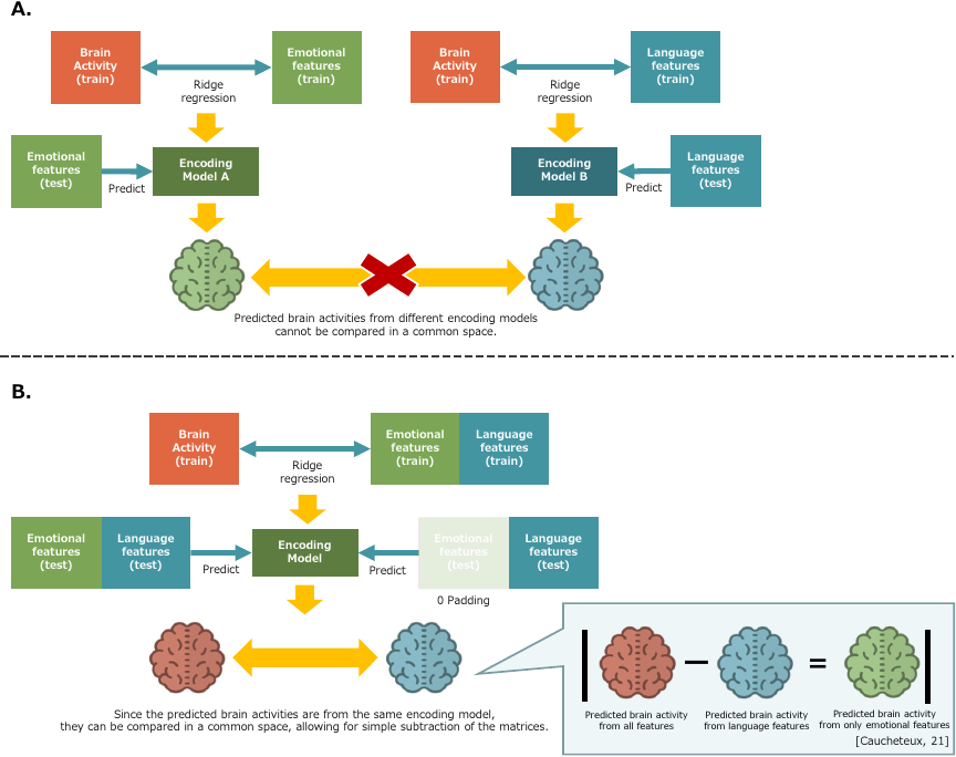
Fig. 1. Regression of both emotional and linguistic features together. A. If brain states are predicted separately from each feature, the predictions cannot be compared in a common space. B. If ridge regression is performed on the combined features and differences between predictions are computed, then predictions are obtained in a common space. Thus, the predicted brain activity based solely on emotional features can be obtained by subtracting the prediction based on language features from the prediction based on all features (matrix subtraction). At the prediction stage on test data, all 80 emotion features linked to the test data were set to 0, and the predicted brain activity from language features was obtained using the constructed encoding model.
4.2.2. Le Petit Prince: A Multilingual fMRI Corpus Using Ecological Stimuli
Le Petit Prince 16 is a dataset published on OpenNeuro that measures brain activity while 49 native English speakers (30 females and 19 males) listen to an audiobook of The Little Prince, translated by David Wilkinson and read aloud in English by Karen Savage. Brain activity during audiobook listening was measured using fMRI to observe BOLD signals in the brain. Brain activity data were collected at 2 s intervals, with each observation volume consisting of \(72 \times 72 \times 33\) (\(=171\mbox{,}072\)) voxels. The 94 min audiobook was divided into nine sections, and brain activity was measured for approximately 10 min in each section. Participants passively listened to one section of the audiobook in each session and answered four questions (36 questions in total) after each session.
4.3. Feature Extraction
Each sentence in the readings was transcribed, and linguistic and emotional features were extracted. As linguistic features of speech content, [CLS] embedding vectors (i.e., BERT’s special classification token representations) were extracted for each sentence using bert-base-cased, a pre-trained BERT model. As the emotional features of speech content, the sigmoid outputs for each emotion were extracted for each sentence using the emotion recognition model constructed in Section 3.2.
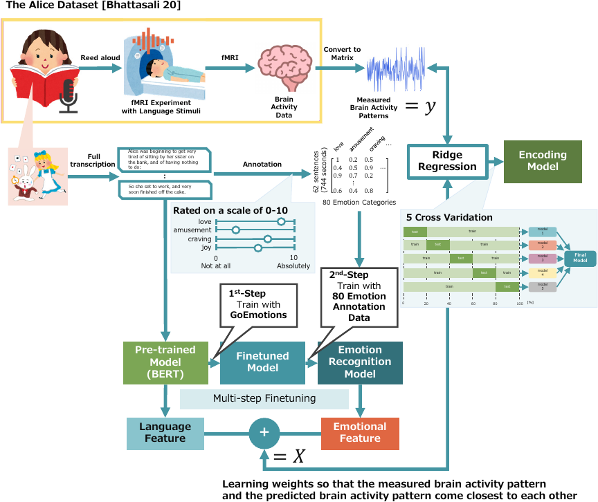
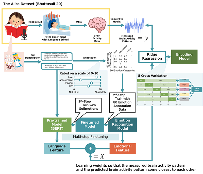
Fig. 2. Overview of constructing encoding models. A. Preprocessing of brain activity data: fMRI datasets collected while humans were listening to narrative readings, such as the Alice dataset, were converted into two-dimensional matrices (\(=y\)). B. Constructing an emotion recognition model: The emotion recognition model was constructed by fine-tuning pre-trained BERT with GoEmotions and further fine-tuning it with 80 emotion annotation data. The transcripts of the full texts read in the Alice dataset were scored by annotators based on how well the 80 emotions matched the emotions they felt when reading each sentence, and then organized as 80 emotion annotation data. C. Extracting features: As language features of speech content, [CLS] embedding vectors were extracted for each sentence using the bert-base-cased, a pre-trained BERT model. As the emotional features of speech content, the sigmoid outputs for each emotion were extracted for each sentence using the emotion recognition model. Then, language and emotional features were concatenated (\(=X\)). D. Constructing encoding models: Encoding models were constructed by performing ridge regression using \(X\) and \(y\). Weights are learned such that the measured and predicted brain activity patterns are close to each other. Because the choice of test data may have caused bias in the results, the test data were swapped among the brain activity datasets, and ridge regression and cross-validation were performed to ensure that the constructed model did not overfit.
4.4. Prediction of Brain States Based on Emotion-Related Features
Because the pre-trained BERT was fine-tuned in multiple steps, the features extracted by the emotion recognition model contained both emotion and language-related information. Based on the idea that purely emotional components can be obtained by removing language-related components from representations 17, we examined differences in brain activity states predicted from each feature set. Fig. 1 presents an overview of this process.
4.5. Experimental Settings
As explained in Section 4.3, language features are extracted from each sentence, and a regression model is constructed using the measured brain activity data. Fig. 2 presents an overview of this process.
4.5.1. Preprocessing and Surface-Based Representation
The present study relies on publicly available fMRI datasets distributed via OpenNeuro. Standard preprocessing steps, including motion correction, slice-timing correction, spatial normalization, and temporal filtering, were performed by the original dataset providers as part of the publicly released datasets. Therefore, our analysis begins with these preprocessed volumetric fMRI data. For surface-based analysis and visualization, we applied cortical surface reconstruction using FreeSurfer’s recon-all pipeline for each subject. This procedure includes skull stripping, tissue segmentation, cortical surface reconstruction, and anatomical labeling. The resulting cortical surfaces were then imported into the PyCortex framework. To align the functional data with the reconstructed cortical surfaces, volume-to-surface projection was performed using pycortex with boundary-based registration. Functional time series were sampled from the volumetric fMRI data onto the cortical surface using a nearest-line mapping approach, yielding vertex-wise cortical activity time courses for each subject. All preprocessing and projection steps were performed using established neuroimaging software packages. Detailed descriptions of these procedures are available in the official documentation of OpenNeuro, FreeSurfer (https://surfer.nmr.mgh.harvard.edu/fswiki/recon-all), and pycortex. For reproducibility, the exact scripts used in this study are publicly available in our GitHub repository (https://github.com/miuraeri/encoding-model-for-emotion/tree/main).
4.5.2. Construction of Encoding Models
In this study, ridge regression was adopted as an encoding model to predict brain states expressed by brain activity data measured by fMRI from spoken content features. For the regularization hyperparameter \(\alpha\) in ridge regression, 15 values of \(\alpha\) between \(10^{-5}\) and \(10^{10}\) were evaluated, and the \(\alpha\) with the highest average correlation coefficient (best alpha) was selected. In the Alice dataset, the brain activity data of each subject was divided into five parts, paying attention to sentence boundaries, and five-fold cross-validation was performed with the test split fixed. As the choice of test data may cause bias in the results, the test split was swapped among the five subsets, and ridge regression and five-fold cross-validation were performed four additional times to ensure that the constructed model did not overfit. In Le Petit Prince, since brain activity data were saved for each session (nine sessions in total), nine-fold cross-validation was performed in the same way as above, with the test split fixed. Thus, five encoding models were constructed for each subject in the Alice dataset, while nine encoding models were constructed for each subject in the Le Petit Prince dataset; however, the best alpha was selected separately for each model. For regression, the temporal delay between the auditory stimulus processing and the observed BOLD response was addressed by concatenating the features and brain activity with multiple time shifts (4, 6, 8, and 10 s). This time-lagged feature construction allowed the linear regression model to capture delayed neural responses without explicitly assuming a fixed hemodynamic response function. In machine learning, data are typically shuffled to suppress overfitting. However, because fMRI data are time-series data, simple random shuffling would disrupt temporal structure. Therefore, contiguous 50 s chunks were created and shuffled as units, preserving local temporal dependencies while reducing overfitting. The model performance was evaluated using Pearson’s correlation coefficient between the predicted and measured BOLD signals for each voxel. Voxel-wise statistical testing was performed against the null hypothesis that the correlation was zero, and \(p\)-values were corrected for multiple comparisons using the false discovery rate (FDR). In addition to the mean correlation coefficients, the variability across subjects and cross-validation folds were quantified using standard deviations, providing reproducibility measures of encoding performance (see Table 4).
Table 4. Values indicate the mean Pearson’s correlation coefficient (\(\rho\)) across voxels (standard deviation in parentheses) and the percentage of significantly predicted voxels after FDR correction.

4.5.3. Average Predicted Brain Activity Across All Subjects and by Gender
To investigate overall subject tendencies and gender differences in emotion-based predicted brain activity, we obtained the average predicted brain activity for all subjects and for males and females separately. However, the predicted brain activity of each subject is a two-dimensional (2D) matrix of time \(\times\) number of voxels. Because the number of voxels differs across subjects, it is difficult to directly average across subjects. When visualizing the predicted brain activity obtained from the constructed encoding model, an arbitrary subject’s (sub-22) flatmap was selected, and the predicted brain activity of each subject was transcribed onto that subject’s flatmap. During the transcription process, the predicted brain activity matrix for each subject (time \(\times\) number of voxels) was transformed into a matrix of time \(\times\) number of voxels for the reference subject (sub-22). The average predicted brain activity for all subjects and for each gender can then be obtained by averaging the post-transcription flatmap matrices of the predicted brain activity based only on the emotional features for each subject.
To assess whether the choice of the reference subject could bias the visualization or the group-level averages, we quantified inter-subject transformability using a “round-trip” correlation test. For each subject, we projected the predicted activity from all other subjects onto that subject’s cortical surface, and then projected it back to the original surface, computing voxel-wise correlations between the original and round-tripped maps. All subjects exhibited uniformly high correlations (close to 1.0) across the cortex, as shown in Fig. 3, with only sparse and very small deviations. These results confirm that individual differences in cortical geometry introduced only negligible distortions. Thus the selection of sub-22 as the reference flatmap does not affect the validity of the group-level visualization or averaging.
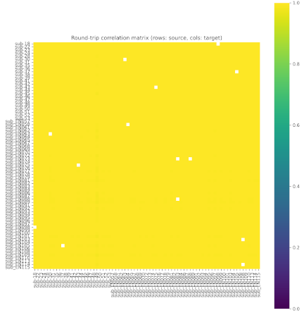
Fig. 3. Round-trip correlation matrix across subjects.
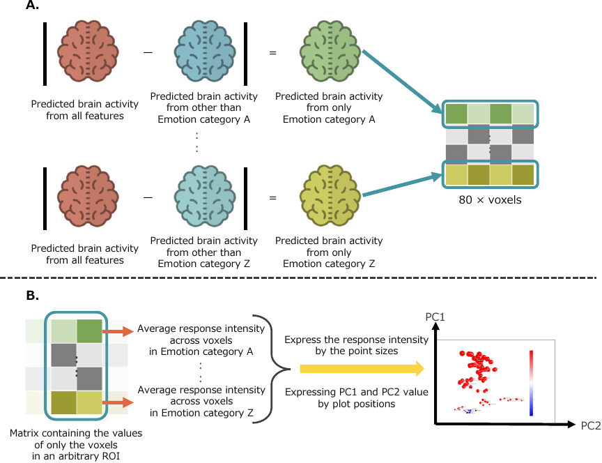
Fig. 4. Response intensity of each emotion by region of interest. A. Following the method shown in Section 4.4, each emotion feature was set to 0, and the predicted brain activity from all other features was obtained using the constructed encoding model. Then, the prediction based solely on each emotion for each subject was obtained by subtracting this from the prediction based on all features. Using the flatmap transformation matrix obtained in the same procedure as described in Section 4.5.3, we averaged the emotion-only predictions across all subjects and time points, and concatenated the matrices for each emotion. In this way, a matrix of 80 (number of emotions) \(\times\) number of voxels is obtained. B. From the matrix described in A, dimensionality reduction to two dimensions was performed using PCA based on a matrix extracted from only the voxels belonging to each region of interest (ROI). The results were projected onto a two-dimensional (2D) space. Emotion categories with similar principal component values are closer in the 2D space. The size of each emotion category point corresponds to the average response intensity of all voxels belonging to the ROI of the category.
4.5.4. Prediction of Brain States Based on Emotional Clusters
Using the weights for each emotion obtained from the encoding model constructed for each subject in the Alice dataset, dimensionality reduction to three dimensions was performed using principal component analysis (PCA). The values of each principal component for each emotion category were assigned to a single color as RGB values and projected onto a 2D space. Emotion categories with similar principal component values were assigned similar colors, and the distance between categories was also small. The size of each point representing an emotion category corresponded to the average weight of the category across all voxels. By clustering using the \(k\)-means method with \(k=6\), the 80 emotion categories were divided into six clusters. For clusters with more than 20 elements, clustering was performed with \(k=2\), and this was set as the final number of clusters.
Brain activity related only to emotions was predicted using the method described in Section 4.4. Similarly, following the method described in Section 4.4, each emotional feature belonging to the clusters was set to 0, and the predicted brain activity from all other features was obtained using the encoding model constructed using the Alice dataset. Then, the predicted brain activity based solely on each cluster was obtained by subtracting the predicted brain activity from all features.
4.5.5. Representational Dissimilarity Analysis
-
1.
RDM1: Time–time representational structure
For each ROI and participant, we computed a time-by-time representational dissimilarity matrix (RDM1). Let \(X \in \mathbb{R}^{T \times V}\) denote the predicted emotion-related neural activity for a given ROI, where \(T\) is the concatenated number of time points across all runs and \(V\) is the number of (masked) voxels. The dissimilarity between time points \(t_i\) and \(t_j\) was quantified using the correlation distance:
\begin{equation} \mathrm{RDM1}(i,j) = 1 - \mathrm{corr} \left(X_{t_i}, X_{t_j} \right). \end{equation}The condensed upper-triangular portion of each RDM1 was vectorized to represent the internal representational geometry of each ROI.
-
2.
RDM2: ROI–ROI representational similarity
To assess the similarity between ROIs, Spearman correlations were computed between the vectorized RDM1s. For ROIs \(r\) and \(q\), the ROI–ROI representational similarity matrix RDM2 was defined as:
\begin{equation} \mathrm{RDM2}(r,q) = \rho \left( \mathrm{vec}\left(\mathrm{RDM1}_r \right), \mathrm{vec} \left(\mathrm{RDM1}_q \right) \right), \end{equation}where \(\mathrm{vec}(\cdot)\) extracts upper-triangle elements. Group-level RDM2 matrices were obtained by averaging the RDM2 across participants within each demographic group (men, women, and all).
-
3.
Network construction and hub identification
Edge selection: Because the ROI–ROI similarity matrix (RDM2) was fully connected, a sparse representational network was constructed by retaining, for each ROI, the two strongest similarity edges (i.e., \(k = 2\) fixed). Formally, for each ROI \(i\), the top two off-diagonal similarity values in row \(i\) were selected, and an undirected adjacency matrix was obtained as:
\begin{equation} A_{ij} = \max\left( w_{i\to j},\ w_{j\to i} \right). \end{equation}PageRank-based hub identification: PageRank scores were computed on the weighted adjacency matrix to identify ROIs that served as global representational hubs—regions receiving strong connections from other strongly connected ROIs.
Visualization: Networks were visualized using a spring layout. Node color and size reflected PageRank values, while node labels displayed the degree of each ROI (number of top-two edges). Labels were rendered with a white outline to ensure readability in the presence of overlapping edges.
4.5.6. Intensity of Emotional Responses by Region of Interest for All Subjects
Using the method described in Section 4.4, each emotion feature was set to 0, and the brain activity predicted from the other features was obtained via the encoding model. The emotion-related predicted activity for each subject was calculated by subtracting this from the full prediction. After applying the flatmap transformation from Section 4.5.3, we averaged these predictions across subjects and time points, then combined them into an 80 (emotions) \(\times\) voxel matrix. PCA reduced this matrix to two dimensions for each ROI, projecting emotions into a 2D space where similar emotions cluster. The point size reflects the average response intensity. See Fig. 4 for an overview.
4.5.7. Evaluation Metrics
The data predicted by the regression model and the actual brain activity data (true data) were evaluated using Pearson’s correlation coefficient. Given the mean values of the true labels and predicted values as \(\bar{y}\) and \(\bar{p}\), respectively, the following equation is used:
A higher positive correlation indicates better predictive accuracy of the encoding model. For each voxel, the statistical significance of the correlation was assessed using a two-tailed hypothesis test under the null hypothesis that there was no correlation between the predicted and true signals (\(p < 0.05\)). To account for multiple comparisons across voxels, FDR correction was applied using the Benjamini–Hochberg procedure. Encoding performance was summarized at the dataset and ROI levels using the following statistics: (1) the mean and standard deviation of Pearson’s correlation coefficients across voxels (before and after FDR correction), and (2) the percentage of voxels showing statistically significant correlations after FDR correction.
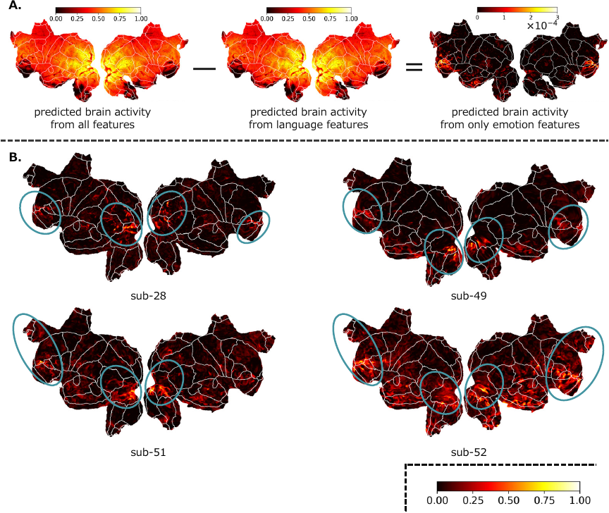
Fig. 5. Brain activity related solely to emotions (the Alice dataset). A. The predicted brain activity when regression was performed combining the emotional and language features for subject sub-30, the predicted brain activity from language features, and the predicted brain activity related only to emotional features. B. The predicted brain activity related solely to emotional features, obtained by subtracting the predicted brain activity related to linguistic features from the predicted brain activity obtained by regressing emotional features and language features for several subjects (sub-28, sub-49, sub-51, sub-52). The blue circles indicate areas that are particularly vigorous. For visualization, values were linearly normalized to the range \([0, 1]\) using min–max normalization for each subject.
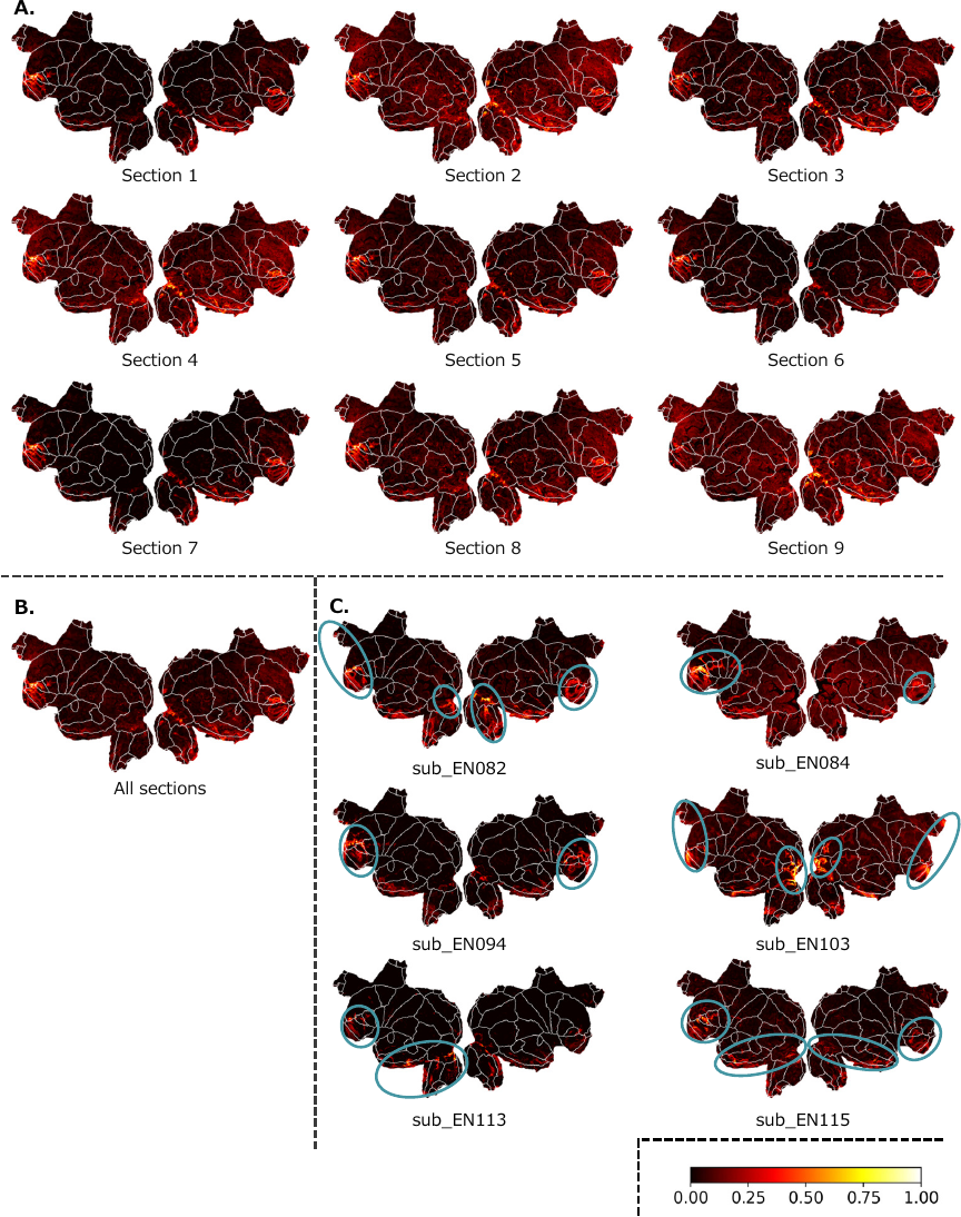
Fig. 6. Brain activity related solely to emotions (Le Petit Prince). The average emotion-related brain activity was related only to the emotional features in Le Petit Prince. For visualization, values were linearly normalized to the range \([0, 1]\) using min–max normalization for each subject: A. for each section (sub-EN058), B. all sections (sub-EN058), and C. results for several subjects (sub-EN082, sub-EN084, sub-EN094, sub-EN103, sub-EN113, sub-EN115). The blue circles indicate areas that were particularly vigorous. Although there are slight differences between sections and subjects, strong reactions were observed in areas related to emotions.
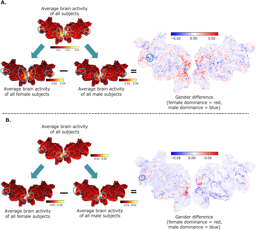
Fig. 7. Average predicted brain activities for all subjects / separated by male and female. The average predicted brain activity based solely on emotions for all subjects and by gender. A. Alice dataset. B. Le Petit Prince dataset.
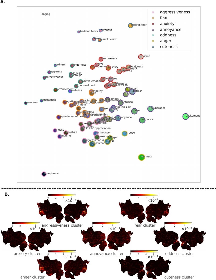
Fig. 8. Mapping of 80 emotion categories and predicted brain activities for each emotion cluster (sub-30). A. Mapping of 80 emotion categories and their clusters onto a 2D space. Each cluster is named after the emotion category closest to the median position of that cluster. B. Predicted brain activity based on emotion-related features belonging to each cluster.
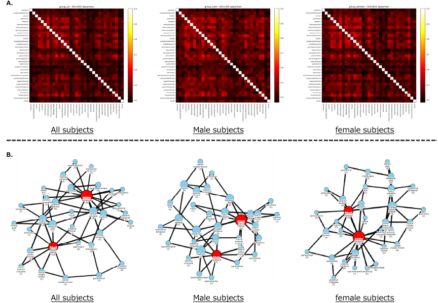
Fig. 9. ROI-based representational similarity and network connectivity for emotion-related brain activity. A. ROI–ROI representational similarity matrices (RDM2) for all, male, and female subjects. Each matrix shows the Spearman correlation between the upper-triangular components of ROI-specific time–time representational dissimilarity matrices (RDM1). Higher values indicate stronger similarity in the temporal structure of emotion-related predictive activity between pairs of ROIs. Across all groups, broadly positive correlations were observed, suggesting a distributed organization of emotion-encoding responses across the cortex. Subtle differences between male and female participants are visible in the fine-grained similarity structure, motivating the network-level analyses presented in panel B. B. Connectivity graphs derived from the ROI–ROI similarity for all, male, and female subjects. Each graph links every ROI to its two most similar ROIs based on the group-averaged RDM2 similarity matrix (nearest-neighbor approach). Nodes represent cortical ROIs, with node labels indicating the ROI name and its degree (number of edges). Red nodes indicate regions with the highest PageRank centrality within each network. Across all groups, the inferior temporal cortex consistently emerged as the primary hub, forming the core of a distributed emotion-encoding network. Secondary hubs differed by group: in all and male subjects, the lateral orbitofrontal cortex showed a relatively high degree, while in female subjects the secondary hub shifted toward the lateral occipital cortex. These graphs illustrate both the shared architecture of the putative affective core network and group-level differences in its topological organization.
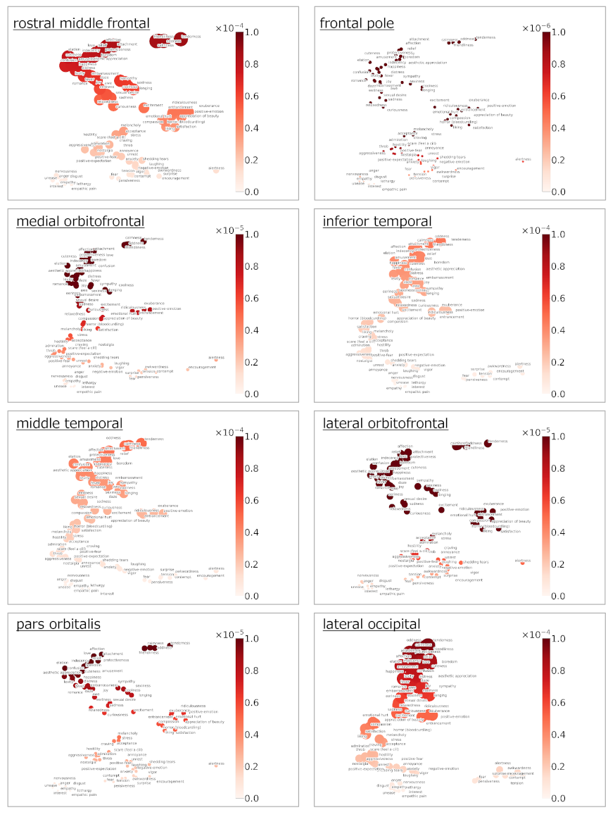
Fig. 10. Intensity of emotion-related responses by region of interest.
4.6. Experiment: Visualization Results
The predicted brain activities related only to emotions for each fMRI experiment are shown in Fig. 5 (Alice dataset) and Fig. 6 (Le Petit Prince dataset). The average predicted brain activities for all subjects, separated by males and females in each experiment, are shown in Fig. 7. The clustering result on 80 emotion categories and the predicted brain activities specific to each cluster are shown in Fig. 8. The ROI–ROI representational similarity matrices for all, male, and female subjects are shown in Fig. 9(A). The corresponding network visualizations based on the top-\(k\) nearest ROI connections (with \(k=2\)) are presented in Fig. 9(B). The intensities of emotional responses by ROI for all subjects are shown in Fig. 10. The quantitative evaluation results of the emotion-based encoding model are summarized in Table 4, which reports the mean and standard deviation of voxel-wise Pearson’s correlation coefficients, as well as the percentage of voxels showing statistically significant prediction accuracy after FDR correction for all voxels and each ROI in both datasets. The visualization results are discussed in detail in the next section.
4.7. Discussion
4.7.1. Stability Improvement of Encoding Accuracy with FDR-Based Voxel Selection
In the Alice dataset, we quantified the fold-to-fold stability in voxel-wise prediction by evaluating the mean Pearson’s correlation coefficient for each subject. Before FDR correction, the mean correlation coefficient across subjects was 0.01297 with a between-subject standard deviation (SD) of 0.03161. The within-subject fold variability was relatively high (mean within-subject SD \(= 0.08175\), SD \(= 0.04268\)), reflecting instability across the five folds, particularly for subjects whose correlations were close to 0. After FDR correction, the mean correlation coefficient increased to 0.09201, and the between-subject variability decreased to 0.02287. Fold-to-fold variability was also reduced (mean within-subject SD \(= 0.04488\), SD \(= 0.02342\)), indicating that thresholding based on statistical significance stabilized the correlation estimates across folds. These results show that in the Alice dataset, FDR correction substantially improved both the magnitude and stability of the mean correlation coefficient.
A similar pattern was observed in the Le Petit Prince dataset. Before FDR correction, the mean correlation coefficient was 0.01162, with a between-subject standard deviation of 0.01330. The within-subject fold variability was moderate (mean within-subject SD \(= 0.03931\), SD \(= 0.01397\)). Some folds yielded no significant voxels prior to FDR correction, resulting in NaN values; these were replaced with 0 to compute for group statistics. After FDR correction, the mean correlation coefficient increased to 0.05541, while the between-subject variability decreased to 0.00825. Fold-to-fold variability was also reduced (mean within-subject SD \(= 0.02656\), SD \(= 0.00676\)). Thus, the FDR correction improved both the magnitude and consistency of voxel-wise correlation coefficients across folds, which is consistent with the findings from the Alice dataset.
Across both narratives, FDR correction increased the mean correlation coefficient and reduced the fold-wise variability. These results indicate that FDR-based voxel selection effectively suppressed noisy voxel contributions and enhanced the robustness of voxel-wise predictions across subjects and stimulus domains.
To evaluate the voxel-wise prediction performance of the encoding model, we computed the correlation between the predicted and measured BOLD responses for each subject and fold, and performed voxel-wise statistical testing against the null hypothesis that the prediction–BOLD correlation was 0. \(p\)-values were corrected for multiple comparisons using FDR, and the proportion of voxels in which the null hypothesis was rejected (significant voxels) was calculated for each fold and averaged within the subjects. Across all subjects, the encoding model produced a remarkably high proportion of significant voxels for both narrative stimuli. For Alice, the mean percentage of significant voxels was 98.56817% (SD \(= 0.26163\)) across subjects. The within-subject variability across the five cross-validation folds was extremely small, with a mean within-subject SD of 0.30951% (SD \(= 0.15355\)). For Le Petit Prince, the mean significant-voxel percentage was slightly lower, but still highly robust, at 96.56169% (SD \(= 0.55566\)). Although Le Petit Prince exhibited slightly more variability across folds and subjects, more than 96% of cortical voxels showed significant prediction performance. Taken together, these findings demonstrate that the proposed encoding model achieves stable and widespread predictive performance across the cortex.
4.7.3. Average Brain Responses of All Subjects and Gender Differences
The analysis of the average predictive brain activity for all subjects and for each gender revealed robust responses across several regions commonly associated with affective processing, including the medial orbitofrontal cortex, frontal pole, lateral orbitofrontal cortex, and rostral middle frontal gyrus. In addition to these canonical affective regions, strong activation was observed in the lateral occipital cortex, suggesting that higher-level visual areas may contribute to emotion representation, possibly through imagery- or perception-based components of affective experiences 23. Importantly, the lateral occipital cortex was not uniquely dominant but instead constituted one of several regions showing strong predictive responses. The relative magnitude of these regional responses are quantified in Fig. 10, which summarizes the voxel-wise response intensities across all ROIs. This pattern indicates that emotional information is embedded within a distributed cortical system, spanning both affective and perceptual regions.
Regarding gender differences, a higher proportion of female-dominant voxels was observed in the orbitofrontal cortex and lateral occipital gyrus across datasets. Meanwhile, male-dominant responses were observed in the left inferior frontal gyrus (Alice dataset) and left middle frontal gyrus (Le Petit Prince dataset). Lateralized patterns emerged in the Le Petit Prince dataset, with stronger predicted responses in the left hemisphere for both overall and gender-specific averages, suggesting a possible hemispheric asymmetry in emotional processing.
4.7.5. Inter-Regional Connectivity of Emotion-Encoding Activity
To characterize how emotion-related predictive activity is coordinated across cortical regions, we computed ROI–ROI representational similarity matrices (RDM2; Spearman correlation of time–time RDMs) and derived sparse connectivity graphs by linking each ROI to its two nearest neighbors in the group-averaged similarity structure (Fig. 9). Panel A shows the ROI–ROI similarity matrices for all, male, and female subjects, while panel B illustrates the corresponding networks. Across all subjects, the RDM2 revealed broadly positive correlations among most ROIs, indicating a widely distributed emotion-encoding architecture. In the corresponding network, the inferior temporal cortex emerged as the most connected hub, exhibiting the highest degree (degree \(=16\)) and PageRank centrality. This region is well known for high-level visual and semantic processing, and its centrality suggests that emotionally relevant representations depend on integrative processes that bridge perceptual and conceptual systems. The lateral orbitofrontal cortex formed a secondary hub (degree \(=10\)), indicating its role in value-related appraisal and flexible evaluation of affective stimuli. Together, these regions form the backbone of an extended affective representational network rather than a modular or anatomically circumscribed system. When the analysis was performed separately for male and female participants, the overall pattern of ROI–ROI similarity was largely preserved, but the network organization showed systematic differences. In male subjects, the inferior temporal cortex again appeared as a central hub (degree \(=7\)), and the lateral orbitofrontal cortex showed higher centrality than in female subjects (degree \(=12\)), suggesting a greater reliance on evaluative or goal-oriented components of affective processing. In contrast, in female subjects, the inferior temporal cortex remained the primary hub (degree \(=17\)), while the lateral occipital cortex, rather than the lateral orbitofrontal cortex, acted as the main secondary hub (degree \(=10\)), which may indicate relatively enhanced integration of affective and perceptual processes. Thus, while both sexes shared a common hub in the inferior temporal cortex, the secondary convergence point of the network differed, with a frontal association node (lateral orbitofrontal) and high-level visual node (lateral occipital) in males and females, respectively. These differences were modest but suggest that gender-related variation in emotion representation may arise not from shifts in which regions are active, but from how representational information flows within the broader cortical network. Taken together, these findings extend prior work on the affective core network by providing a representational-level account of how distributed cortical regions jointly encode emotional information. The combination of cluster-level mapping, voxel-level prediction, and ROI-level network analysis suggests that emotion-related representations are supported by a widespread, hierarchically organized cortical system whose structure is stable across individuals yet shows measurable population-level variation.
4.7.6. Response Intensity of Each Emotional Category
We examined the response intensity of 80 emotion categories across eight cortical ROIs in two narrative-based fMRI experiments using the Alice and Le Petit Prince datasets. Across ROIs, emotion–response profiles were largely similar, suggesting that emotion-related representations under language-driven narrative stimulation were broadly distributed across cortical systems. Although modest regional biases were observed; for example, orbitofrontal regions showing relatively stronger responses to affiliative and socially positive emotions, these differences were quantitative rather than qualitative. Temporal regions exhibited comparable response profiles consistent with their involvement in semantic processing and narrative integration rather than selective engagement by particular emotion categories. Overall, the present results do not support a strongly localized mapping between individual emotion categories and specific cortical regions. A critical factor in interpreting these findings is the nature of the stimuli. Both Alice in Wonderland and Le Petit Prince are narrative texts that predominantly evoke introspective, social, and affiliative emotional states. In contrast, other emotion categories included in the annotation set, such as highly aversive, threat-related, or strongly action-oriented emotions, were likely elicited less frequently or intensely in these narratives. Consequently, the effective sampling of the emotional space is uneven, limiting the extent to which robust conclusions can be drawn about region-specific sensitivity to all emotion categories. Therefore, the absence of strong ROI-specific differentiation should not be interpreted as evidence that such differentiation does not exist in general. Instead, it highlights the importance of stimulus diversity when investigating emotion representations in the brain. To determine whether particular emotions preferentially engaged specific cortical regions, future studies should employ a broader range of linguistic and narrative stimuli that systematically vary in emotional content, intensity, and social context. Taken together, these findings support the view of emotional processing as distributed and context-dependent, with regional differences emerging as graded modulations shaped by the nature of the stimulus. This perspective emphasizes the interaction between emotional category structure, stimulus properties, and cortical function, rather than fixed mappings between discrete emotions and individual brain regions. Comparing our results with those of Koide-Majima et al. 7, which examined emotional responses during video viewing, we observe differences in the cortical regions that exhibited stronger emotion-related responses. While emotion–response profiles within our language-based narrative experiments were broadly similar across ROIs, the ROIs emphasized in video-based studies differ. These discrepancies are likely attributed to differences in stimulus modality (language vs. video) as well as those in encoding model construction and the balance between semantic, perceptual, and affective information processing.
4.7.7. Limitations
Although the present study identified brain regions whose activity was well predicted by emotion-derived features, the observed correlations should be interpreted with appropriate caution. In the encoding-model framework adopted here 6, voxel-wise correlation reflects the degree to which neural responses are predictable from a given feature space, rather than providing direct evidence for the exclusive or causal encoding of a specific psychological construct. Although we aimed to isolate emotion-related information by constructing emotion features and removing linguistic components based on prior work 17, residual contributions from other cognitive processes, such as attention or perceptual factors, cannot be fully excluded. Accordingly, the regions highlighted in our analyses should be understood as emotion-related or emotion-sensitive, rather than strictly emotion-specific. Importantly, voxel-wise statistical testing with FDR correction was applied to control for multiple comparisons to mitigate the risk of false-positive findings. A further limitation is the relatively low performance of the emotion classifier used to extract emotion features. Although this may introduce noise into the subsequent fMRI encoding analysis, the present framework does not rely on accurate discrete emotion identification at the individual trial level. Instead, it aims to capture distributed and continuous emotion-related variance across time and stimuli. The classification accuracy decreases substantially as the number of emotion categories increases, and even established benchmarks with fewer categories report moderate performance. Therefore, the results should be interpreted as reflecting a large-scale representational structure associated with emotion-related signals, rather than the precise decoding of specific emotion labels. Despite this limitation, the resulting encoding and network-level patterns exhibited qualitative consistency with prior neuroimaging findings on emotion processing, suggesting that the extracted features captured meaningful emotion-related variance.
5. Conclusion
In this study, we investigated how emotional meanings embedded in natural language are represented in the human brain. By constructing a multi-step fine-tuned emotion recognition model based on BERT and applying voxel-wise encoding techniques to fMRI data, we extracted emotion-related brain activity after accounting for linguistic features. Rather than revealing strictly localized or category-specific neural substrates, our results indicate that emotional information is represented in a distributed manner across cortical regions, with graded and regionally weighted modulations depending on the emotional content. Specifically, regions such as the orbitofrontal cortex, temporal gyri, and pars orbitalis consistently contributed to emotion-related predictive activity, but without evidence for a one-to-one mapping between individual emotion categories and specific ROI. The organization of emotion-related responses in both the voxel-wise and region-level analyses was consistent with continuous and multidimensional theories of affect, supporting the view that emotional experiences are encoded in a distributed affective space rather than in discrete localized categories, as proposed by prior behavioral and neurocognitive work 2. Beyond the empirical findings, the present study introduces an integrated framework that combines high-dimensional emotion modeling, naturalistic language stimuli, and encoding-based neuroimaging analysis. This framework enables the systematic investigation of how complex emotional structures conveyed by language are reflected in large-scale brain activity. While previous research on emotion representation has focused on visual or facial stimuli, our results highlight that emotionally rich representations also emerge during narrative language comprehension. This underscores the importance of studying emotions in linguistically driven, ecologically valid contexts, where affective meaning unfolds through semantic integration rather than perceptual cues alone. This work demonstrates the feasibility of decoding rich, high-dimensional emotional structures from naturalistic linguistic stimuli and provides a unified framework for disentangling emotion and language-related components of brain activity within an encoding-model approach. The observation of qualitatively similar emotion-related activation patterns across two independent narrative fMRI datasets (Alice and Le Petit Prince), obtained from OpenNeuro under different experimental conditions, supports the robustness and generalizability of the proposed framework. However, several challenges remain. First, emotional processing is inherently dynamic, and future work should incorporate time-resolved modeling to better capture the temporal evolution of affective responses during narrative comprehension. Second, emotional responses to language are likely influenced by individual differences and contextual factors, highlighting the need for personalized models and explicit analyses of inter-subject variability. Finally, because the Le Petit Prince dataset did not include direct emotion annotations, the emotion features for this dataset were inferred using a model trained on the Alice dataset. Future studies should collect emotion annotations for the Le Petit Prince stimuli and perform dataset-specific multistep fine-tuning to enable more direct and balanced comparisons across narratives. In addition, while the present study employed a BERT-based language model to extract emotion-related features, recent work has demonstrated that language models explicitly optimized for brain alignment, such as BrainLM 32, can provide representations that more closely match neural activity patterns. Extending the present framework by fine-tuning brain-aligned language models for emotion representation may further improve encoding performance and provide deeper insights into the neural basis of affective language processing. This represents an important direction for future research.
Acknowledgments
This study was supported by JSPS KAKENHI (Grant Number: 21H05061).
- [1] A. G. Huth, S. Nishimoto, A. T. Vu, and J. L. Gallant, “A continuous semantic space describes the representation of thousands of object and action categories across the human brain,” Neuron, Vol.76, No.6, pp. 1210-1224, 2012. https://doi.org/10.1016/j.neuron.2012.10.014
- [2] A. S. Cowen and D. Keltner, “Self-report captures 27 distinct categories of emotion bridged by continuous gradients,” Proc. of the National Academy of Sciences, Vol.114, No.38, pp. E7900-E7909, 2017. https://doi.org/10.1073/pnas.1702247114
- [3] A. S. Cowen, H. A. Elfenbein, P. Laukka, and D. Keltner, “Mapping 24 emotions conveyed by brief human vocalization,” American Psychologist, Vol.74, No.6, pp. 698-712, 2019. https://doi.org/10.1037/amp0000399
- [4] A. S. Cowen and D. Keltner, “What the face displays: Mapping 28 emotions conveyed by naturalistic expression,” American Psychologist, Vol.75, No.3, pp. 349-364, 2020. https://doi.org/10.1037/amp0000488
- [5] A. G. Huth, W. A. de Heer, T. L. Griffiths, F. E. Theunissen, and J. L. Gallant, “Natural speech reveals the semantic maps that tile human cerebral cortex,” Nature, Vol.532, No.7600, pp. 453-458, 2016. https://doi.org/10.1038/nature17637
- [6] T. Naselaris, K. N. Kay, S. Nishimoto, and J. Gallant, “Encoding and decoding in fMRI,” NeuroImage, Vol.56, No.2, pp. 400-410, 2011. https://doi.org/10.1016/j.neuroimage.2010.07.073
- [7] N. Koide-Majima, T. Nakai, and S. Nishimoto, “Distinct dimensions of emotion in the human brain and their representation on the cortical surface,” NeuroImage, Vol.222, Article No.117258, 2020. https://doi.org/10.1016/j.neuroimage.2020.117258.
- [8] L. A. Wallenwein, S. N. L. Schmidt, J. Hass, and D. Mier, “Cross-modal decoding of emotional expressions in fMRI—Cross-session and cross-sample replication,” Imaging Neuroscience, Vol.2, Article No.imag-2-00289, 2024. https://doi.org/10.1162/imag_a_00289
- [9] S. R. Batten, A. E. Hartle, L. S. Barbosa, B. Hadj-Amar, D. Bang, N. Melville, T. Twomey, J. P. White, A. Torres, X. Celaya et al., “Emotional words evoke region- and valence-specific patterns of concurrent neuromodulator release in human thalamus and cortex,” Cell Reports, Vol.44, No.1, Article No.115162, 2025. https://doi.org/10.1016/j.celrep.2024.115162
- [10] R. Plutchik, “The emotions,” University Press of America, 1991.
- [11] J. A. Russell and L. F. Barrett, “Core affect, prototypical emotional episodes, and other things called emotion: Dissecting the elephant,” J. of Personality and Social Psychology, Vol.76, No.5, pp. 805-819, 1999. https://doi.org/10.1037/0022-3514.76.5.805
- [12] A. C. Weidman, C. M. Steckler, and J. L. Tracy, “The jingle and jangle of emotion assessment: Imprecise measurement, casual scale usage, and conceptual fuzziness in emotion research,” Emotion, Vol.17, No.2, pp. 267-295, 2017. https://doi.org/10.1037/emo0000226
- [13] J. Phang, T. Févry, and S. R. Bowman, “Sentence encoders on stilts: Supplementary training on intermediate labeled-data tasks,” arXiv preprint, arXiv:1811.01088, 2018. https://doi.org/10.48550/arXiv.1811.01088
- [14] V. Kocijan, A.-M. Cretu, O.-M. Camburu, Y. Yordanov, and T. Lukasiewicz, “A surprisingly robust trick for winograd schema challenge,” arXiv preprint, arXiv:1905.06290, 2019. https://doi.org/10.48550/arXiv.1905.06290
- [15] S. Bhattasali, J. Brennan, W.-M. Luh, B. Franzluebbers, and J. Hale, “The alice datasets: fMRI & EEG observations of natural language comprehension,” Proc. of the Twelfth Language Resources and Evaluation Conf., pp. 120-125, 2020.
- [16] J. Li, S. Bhattasali, S. Zhang, B. Franzluebbers, W.-M. Luh, R. N. Spreng, J. R. Brennan, Y. Yang, C. Pallier, and J. Hale, “Le petit prince multilingual naturalistic fMRI corpus,” Scientific data, Vol.9, No.1, Article No.530, 2022. https://doi.org/10.1038/s41597-022-01625-7
- [17] C. Caucheteux, A. Gramfort, and J.-R. King, “GPT-2’s activations predict the degree of semantic comprehension in the human brain,” bioRxiv, 2021. https://doi.org/10.1101/2021.04.20.440622.
- [18] E. T. Rolls, W. Cheng, and J. Feng, “The orbitofrontal cortex: Reward, emotion and depression,” Brain Communications, Vol.2, No.2, Article No.fcaa196, 2020. https://doi.org/10.1093/braincomms/fcaa196
- [19] M. A. J. Apps, M. F. S. Rushworth, and S. W. C. Chang, “The anterior cingulate gyrus and social cognition: Tracking the motivation of others,” Neuron, Vol.90, No.4, pp. 692-707, 2016. https://doi.org/10.1016/j.neuron.2016.04.018
- [20] E. T. Rolls, “Emotion, motivation, decision-making, the orbitofrontal cortex, anterior cingulate cortex, and the amygdala,” Brain Structure and Function, Vol.228, No.5, pp. 1201-1257, 2023. https://doi.org/10.1007/s00429-023-02644-9
- [21] I. Fried, C. L. Wilson, K. A. MacDonald, and E. J. Behnke, “Electric current stimulates laughter,” Nature, Vol.391, No.6668, p. 650, 1998. https://doi.org/10.1038/35536
- [22] M. Belyk, S. Brown, J. Lim, and S. A. Kotz, “Convergence of semantics and emotional expression within the IFG pars orbitalis,” NeuroImage, Vol.156, pp. 240-248, 2017. https://doi.org/10.1016/j.neuroimage.2017.04.020
- [23] S. A. Abdel-Ghaffar, A. G. Huth, M. D. Lescroart, D. Stansbury, J. L. Gallant, and S. J. Bishop, “Occipital-temporal cortical tuning to semantic and affective features of natural images predicts associated behavioral responses,” Nature Communications, Vol.15, No.1, Article No.5531, 2024. https://doi.org/10.1038/s41467-024-49073-8
- [24] C. S. Carver and E. Harmon-Jones, “Anger is an approach-related affect: Evidence and implications,” Psychological Bulletin, Vol.135, No.2, pp. 183-204, 2009. https://doi.org/10.1037/a0013965
- [25] D. Mobbs, P. Petrovic, J. L. Marchant, D. Hassabis, N. Weiskopf, B. Seymour, R. J. Dolan, and C. D. Frith, “When fear is near: Threat imminence elicits prefrontal-periaqueductal gray shifts in humans,” Science, Vol.317, No.5841, pp. 1079-1083, 2007. https://doi.org/10.1126/science.1144298
- [26] D. W. Grupe and J. B. Nitschke, “Uncertainty and anticipation in anxiety: An integrated neurobiological and psychological perspective,” Nature Reviews Neuroscience, Vol.14, No.7, pp. 488-501, 2013. https://doi.org/10.1038/nrn3524
- [27] P. Kuppens, Z. Oravecz, and F. Tuerlinckx, “Feelings change: Accounting for individual differences in the temporal dynamics of affect,” J. of Personality and Social Psychology, Vol.99, No.6, pp. 1042-1060, 2010. https://doi.org/10.1037/a0020962
- [28] D. Keltner and J. Haidt, “Approaching awe, a moral, spiritual, and aesthetic emotion,” Cognition and Emotion, Vol.17, No.2, pp. 297-314, 2003. https://doi.org/10.1080/02699930302297
- [29] G. D. Sherman and J. Haidt, “Cuteness and disgust: The humanizing and dehumanizing effects of emotion,” Emotion Review, Vol.3, No.3, pp. 245-251, 2011. https://doi.org/10.1177/1754073911402396
- [30] L. F. Barrett, “Solving the emotion paradox: Categorization and the experience of emotion,” Personality and Social Psychology Review, Vol.10, No.1, pp. 20-46, 2006. https://doi.org/10.1207/s15327957pspr1001_2
- [31] K. A. Lindquist, T. D. Wager, H. Kober, E. Bliss-Moreau, and L. F. Barrett, “The brain basis of emotion: A meta-analytic review,” Behavioral and Brain Sciences, Vol.35, No.3, pp. 121-143, 2012. https://doi.org/10.1017/S0140525X11000446
- [32] Y. Luo and I. Kobayashi, “Brainlm: Enhancing brain encoding and decoding capabilities with applications in multilingual learning,” J. Adv. Comput. Intell. Intell. Inform., Vol.29, No.4, pp. 754-767, 2025. https://doi.org/10.20965/jaciii.2025.p0754
This article is published under a Creative Commons Attribution-NoDerivatives 4.0 Internationa License.