A Conjugate Gradient-Accelerated Constrained Multi-Objective Optimizer for High-Dimensional Problems with Application to Wellbore Trajectory Planning

Jiafeng Xu; Xin Chen; Yang Zhou

doi:10.20965/jaciii.2026.p0761

single-jc.php

« previous

JACIII Vol.30 No.3 pp. 761-780

(2026)

doi: 10.20965/jaciii.2026.p0761

Research Paper:

Views over last 60 days: 14

A Conjugate Gradient-Accelerated Constrained Multi-Objective Optimizer for High-Dimensional Problems with Application to Wellbore Trajectory Planning

Jiafeng Xu^1,2,3 , Xin Chen^{1,2,3,4,†} , and Yang Zhou^1,2,3

^*1School of Automation, China University of Geosciences
No.388 Lumo Road, Hongshan District, Wuhan, Hubei 430074, China

^*2Hubei Key Laboratory of Advanced Control and Intelligent Automation for Complex Systems
No.388 Lumo Road, Hongshan District, Wuhan, Hubei 430074, China

^*3Engineering Research Center of Intelligent Technology for Geo-Exploration, Ministry of Education
No.388 Lumo Road, Hongshan District, Wuhan, Hubei 430074, China

^*4School of Future Technology, China University of Geosciences
No.388 Lumo Road, Hongshan District, Wuhan, Hubei 430074, China

^†Corresponding author

Received:

October 17, 2025

Accepted:

December 27, 2025

Published:

May 20, 2026

Keywords:

multi-objective optimization, gradient-based optimization, conjugate gradient, wellbore trajectory planning

Abstract

With declining hydrocarbon reserves, optimizing directional wellbore trajectory planning is crucial for accessing complex reservoirs while managing cost and risk. Multi-segment composite trajectories have been widely used in complex formations, but their high-dimensional nature challenges the efficiency of gradient-free multi-objective optimization methods. This paper proposes a conjugate gradient-assisted multi-objective algorithm to accelerate the optimization process. A dual-population update strategy integrates gradient-based search with constraint satisfaction, while adaptive step size and hybrid search mitigate multi-objective gradient conflicts. Gradients for formation-related objectives are approximated via finite differences. The algorithm is validated on a five-segment Bézier trajectory for an extended-reach horizontal wellbore, demonstrating superior normalized hypervolume, convergence, and diversity compared to gradient-based and evolutionary algorithms. Ablation studies verify the effectiveness of the hybrid strategy. The selected trajectory achieves an optimal balance among wellbore length, curvature, and stability under all constraints. To our knowledge, this is the first application of gradient-based multi-objective optimization to wellbore trajectory planning, offering a promising pathway toward real-time drilling trajectory design with enhanced efficiency and robustness.

Multi-objective wellbore path planning

Close full text

Cite this article as:

J. Xu, X. Chen, and Y. Zhou, “A Conjugate Gradient-Accelerated Constrained Multi-Objective Optimizer for High-Dimensional Problems with Application to Wellbore Trajectory Planning,” J. Adv. Comput. Intell. Intell. Inform., Vol.30 No.3, pp. 761-780, 2026.

Data files:

1. Introduction

Directional drilling, a cornerstone technology in modern energy extraction, enables drill bits to navigate around high-risk formations, correct borehole deviations, and access deep targets with significant horizontal reach, and has been widely applied in fields including oil and coal mines ^1,2,3. Recent studies emphasize that achieving economically viable and operationally safe wellbore trajectories demands sophisticated optimization algorithms to balance objectives under nonlinear engineering and geological constraints ⁴. This imperative highlights the need for efficient optimization strategies in deep drilling, where inadequate trajectory designs can introduce uncertainties in directional tracking control, thereby compromising both drilling safety and efficiency ^5,6. This demand is particularly pronounced in high-segment trajectories, which entail numerous decision variables and render current gradient-free methods computationally expensive.

In the early stages of directional drilling planning, gradient-based search methods (e.g., ⁷), particularly the stochastic simplex approximate gradient (StoSAG) algorithm ^8,9, were adopted owing to their mathematical rigor and demonstrated rapid convergence characteristics in idealized computational environments. Notably, Wu and Zhang ¹⁰ developed a switched system framework that transformed wellbore trajectory design into an approximate nonlinear parameter optimization problem, while preserving compatibility with gradient-based solvers through constraint embedding techniques for systematic integration of engineering specifications.

In contrast, gradient-free optimization has become the dominant approach for wellbore trajectory optimization, outperforming gradient-based methods by more effectively handling discrete control variables and non-smooth objective functions inherent to drilling systems. Four main methodological pathways were identified in the literature: (1) classical pattern search algorithms, such as the Hooke–Jeeves method ¹¹, proved effective in combinatorially complex parameter spaces; (2) population-based metaheuristics, including genetic algorithms ^12,13 and particle swarm optimization ^14,15, were widely adopted for their derivative-free evolutionary frameworks; (3) novel heuristics—such as differential search ¹⁶, harmony search ¹⁷, and bio-inspired algorithms like bat optimization ¹⁸ and the spotted hyena optimizer ¹⁹—expanded the methodological spectrum; (4) reinforcement learning (RL) ^20,21 showed potential but remained exploratory due to inefficiencies in its trial-and-error mechanism and strict safety and real-time constraints. Recent trends focused on hybrid approaches (e.g., pattern search-GA integration ²²) and adaptive mechanisms that balanced exploration and exploitation ²³.

The increasing complexity of wellbore trajectory planning also required advanced multi-objective frameworks to balance competing technical and economic criteria. Prior studies extended gradient-free metaheuristics using scalarization techniques to convert multi-objective problems into single-objective formulations ¹⁶, or employed decomposition strategies with Pareto dominance to approximate optimal Pareto fronts ²⁴. Recent developments integrated geological uncertainty quantification ²⁵, spatial constraints ²⁶, and engineering data ⁴ within hybrid optimization architectures. Some research also embedded geomechanical risk models and directional drilling kinematics ²⁷, maintaining computational tractability through adaptive surrogate modeling ²⁸ and parallelized evolutionary operators ²⁹.

Current research exhibits a disproportionate emphasis on gradient-free metaheuristic approaches compared to gradient-based counterparts in wellbore trajectory planning. Despite growing methodological critiques, this trend persists: novel “algorithm zoo”-style evolutionary variants often exhibit zero-biased benchmark behaviors ³⁰. Meanwhile, gradient-based optimization has regained momentum in deep learning through innovations such as normalized least mean square ³¹. In this context, Wood ³² provided the first comparison between generalized reduced gradient (GRG) and GA in the single-objective wellbore trajectory planning cases. Demonstrating 30–\(50\times\) faster computation (3 s vs. 50–100 s per run) while matching GA’s solution quality in most Bézier curve configuration cases, GRG maintained superior efficiency in managing complex drilling constraints like dogleg severity and toolface deviation. This result fundamentally challenges the field’s dominance of gradient-free paradigms, revealing untapped potential in modern gradient-driven optimization frameworks.

Inspired by the above works, this paper aims to bridge this gap by further investigating the effectiveness of various gradient-based multi-objective optimization algorithms in the context of multi-objective wellbore trajectory planning. The main contributions are as follows:

The high dimensionality inherent in multi-segment trajectory optimization is rigorously characterized through an analysis of the degrees of freedom in a composite Bézier curve wellbore trajectory model. This challenge is subsequently addressed by the first application of a gradient-assisted multi-objective optimization method to this problem.
A gradient-based multi-objective algorithm is developed, integrating a dual-population update strategy with an adaptive hybrid search method. This combined mechanism is specifically designed to harness gradient information for accelerated convergence while simultaneously ensuring superior constraint-handling capability and effectively managing conflicting multi-objective gradients.
The efficacy of the proposed method is rigorously validated on a practical multi-formation wellbore trajectory model. Comparative analyses against conventional conjugate gradient methods, steepest descent-based multi-objective optimizers, and state-of-the-art evolutionary algorithms confirm its superior performance.

The remaining sections are structured as follows. Section 2 provides a brief introduction to the problem of multi-objective wellbore trajectory planning in multiple strata, as well as the geometric and geological indicators involved in trajectory optimization. Section 3 presents the multi-dimensional trajectory planning problem and illustrates it with a practical example of extended-reach horizontal wellbore trajectory planning. Section 4 describes the proposed conjugate gradient-based dual-population constrained multi-objective optimization algorithm. Section 5 details the experiments: parameter sensitivity analysis, comparisons with gradient-based and non-gradient algorithms, ablation studies of four variants, performance evaluation of a selected Pareto-optimal trajectory, and its demonstration on a semi-physical platform. Finally, Section 6 provides a discussion, summary, and future outlook.

2. Multi-Objective Wellbore Trajectory Planning in Multiple Strata

Modern directional drilling operations necessitate precise trajectory planning to strike a balance between operational efficiency and downhole safety in complex geological environments.

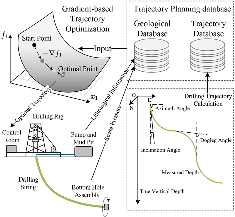
As illustrated in Fig. 1, the directional drilling system consists of surface equipment and downhole tools. The surface installation includes the rig, mud tanks, and control room, which provide power, circulate drilling fluid, and monitor operations. The downhole assembly is composed of the drill string and the bottom hole assembly (BHA). Drilling fluid is pumped through the drill string to cool the bit, carry cuttings to the surface, and help maintain wellbore stability and pressure balance. The BHA is equipped with multiple sensors that gather real-time data on downhole pressure, formation properties, inclination, and azimuth. These engineering and geological measurements are transmitted to the surface via mud pulse telemetry, processed by the programmable logic controller (PLC), and stored in the control room database for analysis and decision-making.

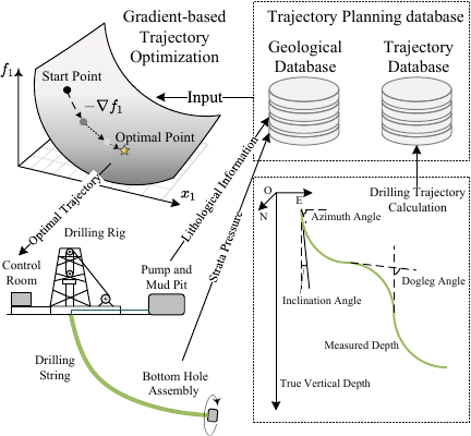
Fig. 1. The process of complex geological directional drilling.

The presence of multiple strata—with abrupt changes in lithology, pore pressure, and formation dip—adds considerable complexity to trajectory design, necessitating adaptive and optimized wellbore trajectory solutions. Using optimization algorithms, a safe and efficient trajectory can be designed and then actively followed through the steering mechanism in the BHA. This facilitates smooth borehole geometry, reduces drilling costs, minimizes friction, and avoids subsurface obstacles. The gradient-based optimization algorithm studied in this paper is specifically developed to support this wellbore planning process.

2.1. Conventional Geometric Indicators of Wellbore Trajectory Planning

Wellbore trajectory planning often uses geometric indicators as objective functions to measure drilling cost and efficiency. The most commonly used geometric indicator is the length of the wellbore trajectory. The length of a composite Bézier curve is approximated using arc length calculation. According to Eq. \(\eqref{eq:tangent_vector}\) (Eqs. (21)–(30) are described in Appendix A), the length of a Bézier curve can be approximated by integrating the magnitude of the tangent vector \(\mathbf{t}(s)\), i.e.,

\begin{equation} L = \int_{0}^{1} |\mathbf{t}(s)| ds. \label{eq:eqbezierarclength} \end{equation}

If the trajectory length is used as the sole optimization objective, it may result in excessive frictional torque on the drill string. To plan smoother trajectories with lower frictional torque, wellbore curvature or torsion is often chosen as a second objective to balance cost and safety. For the Bézier curve \(C(s)\), its curvature and torsion are determined by the derivatives of the path curve:

\begin{equation} \begin{cases} K = \dfrac{|C'(s) \times C''(s)|}{|C'(s)|^3},\\ \tau = \dfrac{\left( C'(s) \times C''(s) \right) \cdot C'''(s)}{| C'(s) \times C''(s) |^2}. \end{cases} \end{equation}

In three-dimensional space, the curvature calculation formula is:

\begin{equation} K = \dfrac{ \sqrt{ \begin{array}{l} \left(C''_D C'_E - C''_E C'_D\right)^2 + \left(C''_N C'_D - C''_D C'_N\right)^2 \\ + \left(C''_E C'_N - C''_N C'_E\right)^2 \end{array} } } { \left(C'_N{}^2 + C'_E{}^2 + C'_D{}^2\right)^{\frac{3}{2}} }, \label{eq:eqbezierK} \end{equation}

where \(C_N\), \(C_E\), and \(C_D\) represent the north, east, and vertical components of the curve, respectively.

2.2. Formation-Related Indicators for Wellbore Trajectory

While geometric indicators facilitate the design of a favorable wellbore trajectory, they inadequately account for formation mechanical properties. This is particularly critical in complex deep formations with heterogeneous lithologies and intricate pressure regimes, where relying solely on geometric parameters may compromise drilling safety and cost-effectiveness. Thus, it is essential to incorporate engineering indicators related to formation characteristics, with wellbore stability being a central concern.

Drilling disturbs the in-situ stress equilibrium. Proper mud density ensures wellbore integrity by balancing formation stresses; insufficient density may cause shear failure and collapse, whereas excessive density can induce tensile fractures. Wellbore stability depends on formation parameters—such as horizontal and vertical stresses, pore pressure, rock strength, friction angle, and Poisson’s ratio—which vary with depth and are intrinsic to the formation. Additionally, wellbore orientation (inclination and azimuth) directly affects stress distribution. Therefore, wellbore stability evaluation must account for the trajectory attitude at each survey point.

Define the function \(\rho(\textit{TVD}, \theta_{inc}, \theta_{azi})\) as the lower-bound safe drilling fluid density required for drilling at vertical depth \(\textit{TVD}\) in the direction specified by inclination angle \(\theta_{inc}\) and azimuth angle \(\theta_{azi}\). This function comprehensively reflects the collapse resistance of the wellbore at that point, resulting from the combined effects of all formation mechanical parameters and trajectory direction.

Considering the multiple formations penetrated by the entire borehole, a comprehensive wellbore stability indicator can be defined as an integrated mapping along the depth direction. Let \(\overline{\rho}(\textit{TVD})\) denote the multi-formation comprehensive wellbore stability indicator at vertical depth \(\textit{TVD}\), representing a generalized measure of the drilling fluid density requirement at that depth across all possible drilling directions. A reasonable definition is:

\begin{equation} \overline{\rho}(\textit{TVD}) = \max_{\theta_{inc},\, \theta_{azi}} \rho\left(\textit{TVD}, \theta_{inc}, \theta_{azi}\right), \label{eq:MultiStrataWS} \end{equation}

i.e., taking the maximum safe mud density among all directions at that depth as the representative stability requirement, thereby ensuring wellbore safety in all orientations. Alternatively, depending on engineering risk preferences, \(\overline{\rho}(\textit{TVD})\) can be constructed using weighted averages or other statistical forms.

3. Medium-to-High Dimensional Composite Wellbore Trajectory Planning

In complex wellbore types such as extended-reach wells and multi-target wells, target segments often reside in geologically intricate formations. To enhance trajectory adaptability, controllability, and engineering feasibility, composite multi-segment curve models are typically adopted to increase design freedom and fitting accuracy, as illustrated in Fig. 14 (in Appendix A). However, each additional curve segment necessitates geometric parameters like azimuth change rate and control point coordinates, thereby increasing decision variables. When geological conditions are extremely complex, multiple targets exist, or displacements are substantial, the number of segments surges, expanding decision variable dimensions to dozens or even hundreds. Consequently, wellbore trajectory planning becomes a medium-to-high-dimensional nonlinear constrained optimization problem, which is demonstrated below through the degrees of freedom (DoF) in composite cubic Bézier curve modeling.

3.1. Degrees of Freedom in Composite Cubic Bézier Curve Trajectory Modeling

In composite cubic Bézier curve trajectory planning, DoF characterizes solution determinacy and optimization potential. For a trajectory comprising \(m\) cubic Bézier segments, the initial control point count is \(4m-2\) (excluding start/end points). Continuity constraints reduce independent control points; \(\mathcal{C}^0\) continuity requires \(m-1\) connection point coincidences, \(\mathcal{C}^1\) continuity adds \(m-1\) tangent vector constraints, and \(\mathcal{C}^2\) continuity with boundary curvature conditions introduces \(m+1\) constraints. With each control point having 3D coordinates \((N, E, D)\), the total DoF equals independent control points multiplied by 3, as shown in Table 1.

Table 1. Composite Bézier curve DoF (\(m\) segments).

When start/end positions are fixed, zero DoF implies a unique solution (e.g., given \(m-1\) target points, a smooth \(m\)-segment trajectory is uniquely determined). Negative DoF indicates over-constrained infeasibility (e.g., \(\mathcal{C}^2\) continuity with \(m=2\) degenerates to a straight line). Positive DoF necessitates optimization to determine the optimal trajectory. For a three-segment curve (\(m=3\)) with fixed endpoints and \(\mathcal{C}^1\) continuity, DoF reaches 18, requiring optimization of at least 18 variables—doubling the scale compared to the 9 variables in the three-segment natural curve model from the previous section.

Critically, DoF directly determines optimization dimensionality. While higher DoF enhances flexibility in satisfying complex geological constraints, it induces a superlinear growth in computational load. For ultra-long horizontal wells or complex 3D multi-target trajectories, segment counts (\(m\)) may exceed 100 segments, resulting in an exponentially heavier computational burden. Under \(\mathcal{C}^0\) and \(\mathcal{C}^1\) continuity, DoF for \(m\) segments is \(6m\). Thus, a 100-segment trajectory planning problem would involve over 600 decision variables, potentially elevating optimization dimensionality to hundreds or thousands of dimensions.

3.2. Extended-Reach Horizontal Wellbore Trajectory Planning

The wellbore trajectory to be planned originates from benchmark extended-reach horizontal wellbore models in studies by Shokir et al. ³³ and Huang et al. ²⁵. While the original case employed conventional tangential-arc trajectory design, this work reconstructs the trajectory using composite cubic Bézier curves to form the continuous smooth drilling path illustrated in Fig. 2.

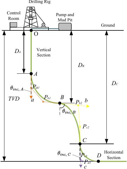
Fig. 2. Multi-segment composite horizontal wellbore trajectory schematic.

Excluding the initial vertical section and target horizontal segment, the build-up sections (\(\widehat{AB}\), \(\widehat{CD}\)) and drop-off section (\(\widehat{BC}\)) are constructed with cubic Bézier curves, requiring \(\mathcal{C}^1\) continuity at composite curve connection points.

According to the \(\mathcal{C}^1\) continuity requirements for composite cubic Bézier curves (Eq. \(\eqref{eq:EqC1continuity}\)), the second control point of each subsequent segment is uniquely determined by the preceding control points. As illustrated in Fig. 2, given the coordinates of control point \(P_{b1}\) and the connection point \(B\), the next segment’s control point satisfies \(P_{b2} = 2B - P_{b1}\), with the remaining second control points determined analogously. Point \(A\) lies on the vertical section at coordinates \((0, 0, D_A)\). Therefore, the complete geometric definition of the wellbore trajectory requires specifying only the following: the third control points (\(P_{c2}\), \(P_{d3}\), etc.) and the coordinates of the connection points (\(B\), \(C\), \(D\)).

Building upon the composite cubic Bézier trajectory model established in Appendix A, the multi-objective optimization model for composite wellbore trajectory planning is formulated as follows:

\begin{align} \begin{aligned} &\min~\left\{ f_1(\mathbf{x}) = L(\mathbf{x}),\ f_2(\mathbf{x}) = \max(K(\mathbf{x})),\ f_3(\mathbf{x}) = \overline{\rho}(\mathbf{x}) \right\}, \\ &\mathrm{s}.\mathrm{t}.~ \left\{ \begin{aligned} & \mathbf{x} = \begin{bmatrix} D_A,\ \mathrm{NED}|_{P_{b1}},\ \mathrm{NED}|_{B},\ \mathrm{NED}|_{P_{c2}}, \\ \mathrm{NED}|_{C},\ \mathrm{NED}|_{P_{d3}},\ \mathrm{NED}|_{D} \end{bmatrix}^{\top}_{\left(19\times1\right)}, \\ & \begin{array}{c@{\;}c@{\;}c@{\;}c@{\;}c} \mathbf{lb}_{P_{b1}} \leq & \mathrm{NED}|_{P_{b1}} \leq \mathbf{ub}_{P_{b1}}, & \quad \mathbf{lb}_{B} \leq & \mathrm{NED}|_{B} \leq \mathbf{ub}_{B}, \\ \mathbf{lb}_{P_{c2}} \leq & \mathrm{NED}|_{P_{c2}} \leq \mathbf{ub}_{P_{c2}}, & \quad \mathbf{lb}_{C} \leq & \mathrm{NED}|_{C} \leq \mathbf{ub}_{C}, \\ \mathbf{lb}_{P_{d3}} \leq & \mathrm{NED}|_{P_{d3}} \leq \mathbf{ub}_{P_{d3}}, & \quad \mathbf{lb}_{D} \leq & \mathrm{NED}|_{D} \leq \mathbf{ub}_{D}, \end{array} \\ & D_A^{\min} \leq D_A \leq D_A^{\max},\ \ \theta_{inc,A} = 0°,\\ & \theta_{azi,A}^{\min} \leq \theta_{azi,A}(\mathbf{x}) \leq \theta_{azi,A}^{\max}, \\ & \begin{aligned} & D_B^{\min} \leq D_B \leq D_B^{\max},\ \ \theta_{inc,B}^{\min} \leq \theta_{inc,B}(\mathbf{x}) \leq \theta_{inc,B}^{\max}, \\ & \theta_{azi,B}^{\min} \leq \theta_{azi,B}(\mathbf{x}) \leq \theta_{azi,B}^{\max}, \end{aligned} \\ & \begin{aligned} & D_C^{\min} \leq D_C \leq D_C^{\max},\ \ \theta_{inc,C}^{\min} \leq \theta_{inc,C}(\mathbf{x}) \leq \theta_{inc,C}^{\max}, \\ & \theta_{azi,C}^{\min} \leq \theta_{azi,C}(\mathbf{x}) \leq \theta_{azi,C}^{\max}, \end{aligned} \\ & \begin{aligned} & \textit{TVD}^{\min} \leq \textit{TVD} \leq \textit{TVD}^{\max},\ \ \theta_{inc,D} = 90°, \\ & \theta_{azi,D}^{\min} \leq \theta_{azi,D}(\mathbf{x}) \leq \theta_{azi,D}^{\max}, \end{aligned} \\ & f_2(\mathbf{x}) \leq K_{\max},\ \ \theta_{inc}(\mathbf{x}) \leq 90°. \end{aligned} \right. \end{aligned} \label{eq:LargeScaleOptimizationModel} \end{align}

The model aims to simultaneously minimize three objective functions: the total trajectory length \(L(\mathbf{x})\) (computed by Eq. \(\eqref{eq:eqbezierarclength}\)), the maximum curvature \(\max(K(\mathbf{x}))\) (computed by Eq. \(\eqref{eq:eqbezierK}\)), and the integrated wellbore stability index \(\overline{\rho}(\mathbf{x})\) (calculated as the mean value from Eq. \(\eqref{eq:MultiStrataWS}\)).

The decision variable \(\mathbf{x}\) is a vector comprising 19 scalar components, where \(\mathrm{NED}|_{P_{b1}}\) denotes the NED coordinates \((N_{P_{b1}},E_{P_{b1}},D_{P_{b1}})\) of the third control point \(P_{b1}\) for the first Bézier curve segment \(\widehat{AB}\). The vector \(\mathbf{x}\) also includes the NED coordinates of other key points (the junction points \(B\), \(C\), the target point \(D\), and the third control points \(P_{c2}\), \(P_{d3}\) for segments \(\widehat{BC}\) and \(\widehat{CD}\)), along with \(D_A\). All decision variables are bounded by predefined constraints (\(\mathbf{lb}, \mathbf{ub}\)). Furthermore, the model incorporates critical engineering constraints: the true vertical depth (TVD) (\(D_A, D_B, D_C, \textit{TVD}\)), inclination angle (\(\theta_{inc, A}=0°, \theta_{inc, D}=90°, \theta_{inc, B}, \theta_{inc, C}\)), and azimuth angle (\(\theta_{azi, A}, \theta_{azi, B}, \theta_{azi, C}, \theta_{azi, D}\)) at the kick-off point \(A\), target point \(D\), and junction points \(B\), \(C\) must satisfy specified upper and lower bounds. Simultaneously, the maximum curvature \(K\) along the entire trajectory must not exceed the maximum build rate capability of the drilling steerable tool, and the maximum inclination angle must be less than \(90°\) to prevent trajectory backtracking.

In summary, this model constitutes a nonlinear constrained multi-objective optimization problem with a 19-dimensional decision variable vector, requiring the simultaneous minimization of three nonlinear objective functions. The high dimensionality of the decision variables and the stringent constraint conditions necessitate that the trajectory planning algorithm possesses the capability to efficiently handle high-dimensional nonlinear space search, satisfy complex engineering constraints, and effectively trade off multiple conflicting objectives.

4. Constrained Multi-Objective Optimization with Conjugate Gradient

Addressing the medium-to-high-dimensional search space characteristic of the trajectory planning problem for large-displacement horizontal wellbore drilling, this section introduces a constrained multi-objective optimization method with conjugate gradient (CMOCG). Regarding the gradient optimization strategy, the conjugate gradient method is employed in conjunction with finite-difference gradient computation. The search direction is adaptively selected based on solution feasibility, utilizing either the objective function gradient or the constraint function gradient. For constraint conflict handling, a dual-population cooperative evolutionary framework is constructed. Conflict symbol labeling is utilized to identify objective conflicts across decision variable dimensions. An adaptive strategy combining conjugate gradient descent and differential gradient direction adjustment is implemented. Furthermore, an acceptance criterion based on constraint violation degree and objective improvement is introduced to ensure efficient convergence within the feasible region while maintaining population diversity.

4.1. Dual-Population Optimization Framework with Conjugate Gradient Assisted Search

Although gradient methods exhibit efficient convergence performance in single-objective optimization, their application to constrained multi-objective optimization problems presents challenges. The inherent conflicts between different objectives often cause a single gradient direction to exhibit gradient conflict, while the introduction of constraints further complicates the determination of effective search directions.

To overcome these difficulties and efficiently solve the high-dimensional wellbore trajectory planning problem, the CMOCG algorithm constructs a co-evolutionary dual-population framework, as illustrated in Algorithm 1. CMOCG employs two populations with differential sizing. The larger main population (\(P_1\)) is assigned the role of maintaining global diversity and convergence, updated through non-dominated sorting and elitist selection mechanisms. In contrast, the smaller auxiliary population (\(P_2\)) focuses on gradient-guided local search, with its reduced size mitigating computational demands in high-dimensional spaces.

During the iterative process, the two populations maintain limited information exchange. If the solution generation process in \(P_2\) fails due to gradient or constraint conflicts, solutions are randomly selected from \(P_1\) to replenish \(P_2\) (Algorithm 1, line 16). Conversely, conflict-free solutions generated within \(P_2\) are directly incorporated into the offspring population (\(\textit{Off}\)). These offspring solutions are then passed to \(P_1\) for further environmental selection via fast non-dominated sorting, enabling cyclic updates of the main population (Algorithm 1, lines 7–19).

In the initialization phase, the CMOCG algorithm generates a uniformly distributed set of weight vectors \(W\) for subsequent objective gradient calculations, while simultaneously initializing the gradient set \(G\), search direction set \(H\), and iteration counter \(K\) to store historical optimization information. During the iterative phase, CMOCG computes the Jacobian matrix via the finite difference method (Algorithm 2) based on solution feasibility status—objective functions for feasible solutions or constraint violation functions for infeasible solutions—yielding gradient \(g_k\) while updating conflict marker \(site\) according to gradient conflict status. The conjugate search direction \(d_k\) is updated as the following expression:

\begin{equation} \label{eq:EqCG} d_{k} = \text{CG}\left(g_k, G[i], H[i]\right) = -g_{k} + \beta_k d_{k-1}, \end{equation}

where \(d_{k-1}\) denotes the previous search direction, with the initial direction set to steepest descent (\(d_0 = -g_0\)). Subsequent iterations compute \(\beta_k\) using the Fletcher–Reeves formula:

\begin{equation} \beta_k^{\mathrm{FR}} = \frac{g_k^\top g_k}{g_{k-1}^\top g_{k-1}}, \end{equation}

(as implemented in Algorithm 1, line 9). CMOCG then executes a variable step-size conflict-handling hybrid search along the selected conjugate gradient direction \(d_k\) (Algorithm 3). If successful in finding an improved feasible solution \(x\) with better convergence, it updates the auxiliary population along with gradients \(G[i]\) and directions \(H[i]\); if unsuccessful, it triggers a fallback operation where the auxiliary population \(P_2\) replaces the individual through random selection from the main population \(P_1\) and resets the counter. All candidate solutions \(\textit{Off}\) generated by the auxiliary population are incorporated into the main population’s candidate pool. Finally, through environmental selection, the main population selects offspring from the merged solution set to ensure convergence toward the Pareto front while maintaining solution diversity.

The constraint handling mechanism is integrated to both population update processes, operating through a systematic evaluation and enforcement protocol. For \(P_2\), constraint evaluation occurs at two critical stages: during gradient selection and solution acceptance. In the gradient calculation phase (Algorithm 2), the constraint violation measure determines the computational pathway, directing infeasible solutions toward constraint satisfaction by following constraint gradient directions while feasible solutions pursue objective optimization. Subsequently, during the adaptive step search (Algorithm 3), newly generated solutions undergo constraint assessment against constraint-domination criteria, where acceptance requires either reduced constraint violation or maintained feasibility with improved objective performance.

For \(P_1\), constraint enforcement occurs during environmental selection. The fast non-dominated sorting procedure incorporates constraint violation as a primary criterion, ensuring that feasible solutions dominate infeasible ones, and among infeasible solutions, those with lower constraint violation are preferred. This dual mechanism ensures progressive movement toward the feasible region while maintaining convergence to the Pareto-optimal front.

4.2. Finite Difference Approximation for Gradient Calculation

For multi-objective optimization problems with general continuous objective functions, the Jacobian matrix \(\nabla \mathbf{obj}\) of objective values can be directly computed through first-order partial derivatives. For the tri-objective optimization problem in Eq. \(\eqref{eq:LargeScaleOptimizationModel}\), this yields:

\begin{equation} \label{eq:EqObjGradient1} \nabla \mathbf{obj} = \begin{bmatrix} \dfrac{\partial f_1}{\partial D_A} & \dfrac{\partial f_1}{\partial N_{P_{b1}}} & \dfrac{\partial f_1}{\partial E_{P_{b1}}} & \dfrac{\partial f_1}{\partial D_{P_{b1}}} & \cdots & \dfrac{\partial f_1}{\partial \textit{TVD}},\\ \dfrac{\partial f_2}{\partial D_A} & \dfrac{\partial f_2}{\partial N_{P_{b1}}} & \dfrac{\partial f_2}{\partial E_{P_{b1}}} & \dfrac{\partial f_2}{\partial D_{P_{b1}}} & \cdots & \dfrac{\partial f_2}{\partial \textit{TVD}},\\ \dfrac{\partial f_3}{\partial D_A} & \dfrac{\partial f_3}{\partial N_{P_{b1}}} & \dfrac{\partial f_3}{\partial E_{P_{b1}}} & \dfrac{\partial f_3}{\partial D_{P_{b1}}} & \cdots & \dfrac{\partial f_3}{\partial \textit{TVD}} \end{bmatrix}. \end{equation}

Similarly, denoting constraint violation functions in Eq. \(\eqref{eq:LargeScaleOptimizationModel}\) as \(h_i\), the Jacobian matrix \(\nabla \mathbf{con}\) for constraint violations is computed as:

\begin{equation} \label{eq:EqConGradient1} \nabla \mathbf{con} = \begin{bmatrix} \dfrac{\partial h_1}{\partial D_A} & \dfrac{\partial h_1}{\partial N_{P_{b1}}} & \dfrac{\partial h_1}{\partial E_{P_{b1}}} & \dfrac{\partial h_1}{\partial D_{P_{b1}}} & \cdots & \dfrac{\partial h_1}{\partial \textit{TVD}},\\ \dfrac{\partial h_2}{\partial D_A} & \dfrac{\partial h_2}{\partial N_{P_{b1}}} & \dfrac{\partial h_2}{\partial E_{P_{b1}}} & \dfrac{\partial h_2}{\partial D_{P_{b1}}} & \cdots & \dfrac{\partial h_2}{\partial \textit{TVD}},\\ \vdots & \vdots & \vdots & \vdots & \ddots & \vdots,\\ \dfrac{\partial h_{17}}{\partial D_A} & \dfrac{\partial h_{17}}{\partial N_{P_{b1}}} & \dfrac{\partial h_{17}}{\partial E_{P_{b1}}} & \dfrac{\partial h_{17}}{\partial D_{P_{b1}}} & \cdots & \dfrac{\partial h_{17}}{\partial \textit{TVD}},\\ \dfrac{\partial h_{18}}{\partial D_A} & \dfrac{\partial h_{18}}{\partial N_{P_{b1}}} & \dfrac{\partial h_{18}}{\partial E_{P_{b1}}} & \dfrac{\partial h_{18}}{\partial D_{P_{b1}}} & \cdots & \dfrac{\partial h_{18}}{\partial \textit{TVD}} \end{bmatrix}. \end{equation}

However, certain objective functions (particularly \(f_3\) related to formation characteristics) and constraint violation functions may exhibit non-smooth properties, making analytical solutions of their partial derivatives intractable. To address this, finite difference methods numerically approximate the Jacobian matrices. For objectives \(\mathbf{obj} = [f_1, f_2, f_3]^\top\), elements are approximated via forward difference:

\begin{equation} \label{eq:EqObjGradient2} \frac{\partial f_k}{\partial x_j} \approx \frac{f_k\left(\mathbf{x}_{j+\epsilon}\right) - f_k(\mathbf{x})}{\epsilon}, \quad k=1,2,3. \end{equation}

Similarly, for constraint violations \(\mathbf{h} = [h_1,\dots,h_{18}]^\top\):

\begin{equation} \frac{\partial h_i}{\partial x_j} \approx \frac{h_i\left(\mathbf{x}_{j+\epsilon}\right) - h_i(\mathbf{x})}{\epsilon}, \quad i=1,\dots,18, \label{eq:EqConGradient2} \end{equation}

where \(\mathbf{x}_{j+\epsilon} = (x_1, \dots, x_{j-1}, x_j + \epsilon, x_{j+1}, \dots, x_n)\) denotes the solution vector perturbed along the \(j\)-th variable dimension, and \(n\) is the total number of design variables. The perturbation step size \(\epsilon\) scales with variable ranges:

\begin{equation} \epsilon = 10^{-6}\left(u_j - l_j\right), \end{equation}

with \(u_j\) and \(l_j\) being the upper and lower bounds of the \(j\)-th design variable.

When solution \(\mathbf{x}\) violates constraints, CMOCG prioritizes constraint violation (CV) reduction over objective optimization to expedite entry into feasible regions. The CV measures the total infeasibility of a solution \(\mathbf{x}\). It is defined as:

\begin{equation} \label{eq:CV} CV(\mathbf{x}) = \displaystyle\sum\limits_{i=1}^{m} \max\left(0, ; c_i(\mathbf{x})\right) + \displaystyle\sum\limits_{j=1}^{p} \left|e_j(\mathbf{x})\right|, \end{equation}

where \(c_i(\mathbf{x}) \leq 0\) are inequality constraints and \(e_j(\mathbf{x}) = 0\) are equality constraints. A solution is feasible if \(CV(\mathbf{x}) = 0\). The algorithm first computes \(\nabla \mathbf{con}\) using Eqs. \(\eqref{eq:EqConGradient1}\) and \(\eqref{eq:EqConGradient2}\) (Algorithm 2, lines 1–4). To ensure equal importance across constraints, a unit weight vector \(\mathbf{1}^\top\) aggregates constraint gradients into \(g_k \gets \mathbf{1}^\top \nabla \mathbf{con}\), while initializing the conflict marker as a zero vector (\(site \gets \mathbf{0}_{Dim}\)).

For feasible solutions, CMOCG computes the objective Jacobian matrix \(\nabla \mathbf{obj}\) using Eqs. \(\eqref{eq:EqObjGradient1}\) and \(\eqref{eq:EqObjGradient2}\) (Algorithm 2, line 6). Unlike the unit vector aggregation for constraint gradients in infeasible solutions, feasible solutions employ a predefined weight vector \(W\) to aggregate objective gradients (\(g_k \gets W^\top \nabla \mathbf{obj}\)). This gradient utilization enhances population convergence while uniformly distributed weight vectors \(W\) guide different solutions toward distinct directions along the Pareto front, thereby maintaining population diversity.

During objective gradient aggregation, CMOCG detects and handles potential gradient conflicts. For the \(j\)-th decision variable, if its partial derivative set \({\partial f_1/\partial x_j, \partial f_2/\partial x_j, \dots, \partial f_M/\partial x_j}\) contains both positive and negative values (i.e., \(\exists k: \nabla \mathbf{obj}{k,j} > 0 \land \exists k: \nabla \mathbf{obj}{k,j} < 0\)), the conflict marker \(site[j]=1\) is activated. This indicates that gradient-based updates along this variable would simultaneously improve certain objectives while deteriorating others. When such conflicts occur, direct application of gradient-based update rules becomes unsuitable. Consequently, CMOCG switches to a random differential strategy to enhance exploration capability and mitigate multi-objective conflicts induced by gradient updates.

4.3. Hybrid Search with Adaptive Step Size for Conflict Handling

After obtaining the search direction \(d_k\) via conjugate gradient calculation (Eq. \(\eqref{eq:EqCG}\)), the auxiliary population \(P_2\) generates new solutions through line search as expressed in Eq. \(\eqref{eq:EqLineSearch}\):

\begin{equation} \label{eq:EqLineSearch} x = P_2[i] + \alpha \cdot d_{k}, \end{equation}

where \(\alpha\) denotes the search step size, the CMOCG algorithm employs an exponential decay mechanism to adaptively adjust \(\alpha\): an initial larger step size (\(\alpha=1\)) is set to enhance global exploration capability; as the iteration count \(step\) increases, the step size \(\alpha\) is gradually reduced until it reaches \(\alpha=0.002\), ultimately focusing on local exploitation. To ensure computational efficiency, the maximum number of step size adjustments \(S_{\max}\) is predefined (Algorithm 3, lines 2–3).

For dimensions flagged with gradient conflicts (\(site=1\)) as described previously, directly applying search direction \(d_k\) may fail to discover improved Pareto solutions; to overcome this issue, CMOCG employs differential mutation introducing stochastic perturbations by randomly selecting two distinct solutions \(\mathbf{x}'\) and \(\mathbf{x}''\) from the main population \(P_1\) (excluding current solution \(P_2[i]\)), generating new solutions via \(x = P_2[i] + \alpha \cdot (\mathbf{x}' - \mathbf{x}'')\), while for non-conflict dimensions (\(site=0\)), stable updates proceed along the predetermined gradient direction \(d_k\) (Algorithm 3, lines 4–11).

Newly generated solutions \(x\) undergo feasibility assessment through constraint-domination criteria: immediate acceptance occurs if \(CV(x) < CV(P_2[i])\), whereas when \(CV(x) = CV(P_2[i])\), acceptance requires \(x\) to be non-inferior to \(P_2[i]\) across all objectives with strict improvement in at least one objective, satisfying the Pareto dominance condition (Algorithm 3, lines 12–14).

5. Experiments

All comparative experiments conducted in this study were performed on the composite cubic Bézier trajectory model for extended-reach horizontal wellbore planning, as detailed in Section 3.2. This model represents a classic and widely adopted wellbore type in practical extended-reach drilling operations. It constructs the trajectory using three cubic Bézier curve segments (\(m=3\)) to model the successive build-up, drop-off, and final build-up sections, ensuring smooth \(\mathcal{C}^1\) continuity at connections. Parameterized by 19 decision variables, including the coordinates of key junction points (\(B\), \(C\), \(D\)) and critical control points (\(P_{b1}\), \(P_{c2}\), \(P_{d3}\)) as defined in Eq. \(\eqref{eq:LargeScaleOptimizationModel}\), this model offers a representative and tractable test case. It was selected for benchmarking primarily because it corresponds to a realistic, commonly drilled wellbore profile with established precedents in the literature ^33,25. Its practical relevance ensures that the optimization challenges are authentic, while its moderate scale provides a feasible yet non-trivial benchmark for comparing multi-objective algorithms. Although higher-dimensional models with more segments could further stress-test algorithmic scalability, such as in complex geo-steering scenarios with frequent directional changes, the current model serves as a robust and standardized basis for initial performance evaluation within the scope of this study. The key point design parameters are as follows:

Point A: Inclination angle \(\theta_{inc, A}\) = 0°, with a true vertical depth (TVD) \(D_A\) ranging from 182.9 to 304.8 meters.
Point B: Inclination angle \(\theta_{inc, B}\) ranging from 10° to 20°, with a TVD \(D_B\) ranging from 1828.8 to 2133.6 meters.
Point C: Inclination angle \(\theta_{inc, C}\) ranging from 40° to 70°, with a TVD \(D_C\) ranging from 3048.0 to 3109.0 meters.
Point D: Inclination angle \(\theta_{inc, D}\) = 90°, with a target TVD ranging from 3307.1 to 3322.3 meters.

Additionally, the azimuth angles at all points are constrained between \(-10°\) and 10°, and the curvature \(K\) along the entire trajectory must not exceed 10° per 30 meters.

5.1. Parameter Settings for Auxiliary Population Size and Maximum Step Size Adjustment Attempts of CMOCG

In the CMOCG algorithm, two parameters significantly influence its performance: the size \(N_2\) of the auxiliary population \(P_2\), which controls the number of individuals performing gradient-guided search, and the maximum number of step size adjustment attempts \(S_{\max}\) in the hybrid search with variable step size for conflict handling, which directly affects the granularity of the local search and the associated computational cost.

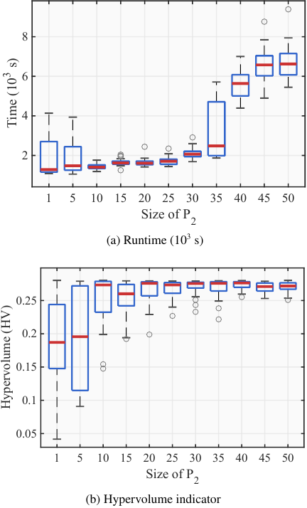
Fig. 3. Performance comparison for different sizes of \(P_2\).

To investigate the impact of the auxiliary population size, the maximum step size adjustment was fixed at \(S_{\max}=10\), while \(N_2\) was set to 1, 5, 10, 15, 20, 25, 30, 35, 40, 45, and 50, respectively. The CMOCG algorithm was employed to solve the extended-reach horizontal wellbore trajectory planning problem under each parameter setting. Each configuration was independently run 30 times, and boxplots of the runtime and normalized hypervolume indicator were generated, as shown in Fig. 3.

From the runtime comparison in Fig. 3(a), it is evident that when \(N_2 \geqslant 40\), the average runtime increases significantly, approximately three times longer than the average runtime for \(N_2 \leqslant 40\), indicating that a huge auxiliary population size substantially increases computational overhead. The distribution of the hypervolume indicator in Fig. 3(b) shows that the mean hypervolume indicator remains largely unchanged for \(N_2 \geqslant 10\), suggesting that blindly increasing the auxiliary population size does not effectively enhance the quality of the solution set. Within the range of \(N_2 \leqslant 10\), although the runtime increases slightly with larger \(N_2\), the hypervolume indicator does not show significant improvement, indicating that expanding the auxiliary population size does not lead to notable enhancements in the algorithm’s diversity and convergence.

Considering both algorithmic efficiency and convergence performance, setting the auxiliary population size to \(N_2=10\) represents an optimal choice for solving the extended-reach horizontal wellbore trajectory planning model in this section, as it ensures satisfactory search effectiveness while controlling computational costs.

To analyze the impact of the maximum number of step size adjustment attempts on algorithm performance, the auxiliary population size was fixed at \(N_2=10\), while \(S_{\max}\) was set to 1, 5, 10, 15, 20, 25, 30, 35, 40, 45, and 50, respectively. The CMOCG algorithm was employed to solve the extended-reach horizontal wellbore trajectory planning problem under each parameter configuration. Each setting was independently run 30 times. The runtime and normalized hypervolume indicator were recorded, and the corresponding boxplots are shown in Fig. 4.

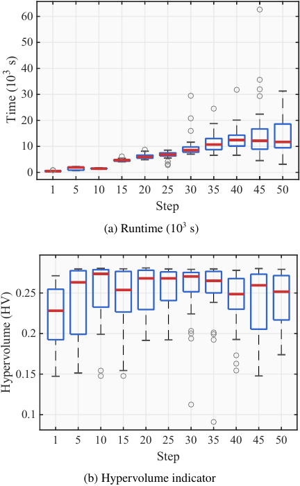
Fig. 4. Performance comparison for different steps.

Table 2. Experimental configuration and algorithm parameter settings.

As can be observed from Fig. 4(a), the algorithm’s runtime exhibits an approximately linear increasing trend with the number of maximum step size adjustment attempts. Fig. 4(b) indicates that the mean hypervolume indicator reaches its maximum at \(S_{\max}=10\), suggesting that the algorithm achieves superior comprehensive search performance under this configuration. Therefore, setting the maximum number of step size adjustment attempts to \(S_{\max}=10\) represents an optimal choice for solving the extended-reach horizontal wellbore trajectory optimization model in this section, as it ensures satisfactory convergence accuracy while effectively controlling computational expenditure.

5.2. Comparison of Hypervolume Metrics Across Competing Algorithms

5.2.1. Experimental Setup and Comparative Algorithms

This section outlines the experimental configuration and introduces the baseline algorithms employed to evaluate the performance of the proposed CMOCG algorithm in the context of trajectory planning for extended-reach horizontal drilling. To ensure a comprehensive comparison, the selected baselines encompass a spectrum of strategies, ranging from pure gradient-based methods to those hybridizing evolutionary and gradient techniques, as well as a canonical gradient-free evolutionary algorithm.

The following algorithms are included in this comparative study:

Multi-Objective Conjugate Gradient (MOCG): A direct extension of the classical conjugate gradient method to multi-objective optimization ³⁴. Unlike CMOCG, it lacks evolutionary mechanisms such as the dual-population framework and gradient conflict detection. Regarding solution update strategies, MOCG adopts a standard line search method with an acceptance criterion based on the Armijo condition: a new solution is accepted for subsequent iterations if it satisfies \(f_{\text{new}} \leq f_{\text{old}} + \sigma \alpha \mathbf{g}_k^\top \mathbf{d}_k\).
Multi-Objective Steepest Descent (MOSD): A special case of MOCG obtained by setting \(\beta = 0\) in the conjugate gradient update formula (Eq. \(\eqref{eq:EqCG}\)), effectively reducing to the steepest descent method in the multi-objective setting ³⁵.
Multi-Objective Aggregative Gradient-Based Optimization (MOAG): An algorithm that employs an aggregative gradient strategy for multi-objective optimization ³⁶.
Multi-Objective Evolutionary Gradient Search (MOEGS): A hybrid algorithm that estimates the Pareto front’s gradient direction via stochastic perturbation sampling and incorporates an adaptive step-size mechanism ³⁷.
NSGA-III: A canonical gradient-free evolutionary algorithm, included as a representative of state-of-the-art multi-objective evolutionary optimizers ³⁸.

To guarantee the fairness and reproducibility of our comparative experiments, the parameter settings for all baseline algorithms were meticulously adopted from their original publications. Furthermore, the specifications of the computational environment are provided. All implementation details necessary to replicate this study are comprehensively summarized in Table 2, located at the end of this subsection. This includes a complete listing of algorithm-specific parameters and their values, all of which are cited to their source literature. A uniform population size of 100 was used across all algorithms, and each was executed independently for 30 runs to ensure statistical significance.

5.2.2. Experimental Results

The computation time and normalized hypervolume metric are recorded, and the results are presented via boxplots in Fig. 5.

As illustrated in Fig. 5(a), all algorithms except MOAG are computationally efficient. The quantitative results from 30 independent runs reveal that MOAG required an average computation time of approximately \(6 \times 10^3\) seconds, whereas the average time for all other algorithms remained below \(2 \times 10^3\) seconds. Notably, the proposed CMOCG was not the fastest algorithm; both MOSD and the gradient-free NSGA-III consistently exhibited lower runtimes. MOEGS was the most computationally efficient, with nearly all executions completing under \(10^3\) seconds, barring minor outliers.

Regarding solution quality, the normalized hypervolume metrics in Fig. 5(b) show that CMOCG achieved the highest average hypervolume (HV) of 0.28, significantly outperforming its competitors. Except for a few runs that fell below 0.2, CMOCG consistently maintained HV above 0.26. Although the absolute difference appears small, a gap of 0.01–0.03 in HV corresponds to a substantial disparity in the actual Pareto front. For instance, NSGA-III, with an average HV of 0.25, exhibited noticeable disadvantages in both diversity and convergence upon visual inspection of the solutions. MOCG also demonstrated reasonable performance with an HV of 0.21, yet a significant gap remains when compared to CMOCG and NSGA-III.

Conversely, the three remaining algorithms (MOSD, MOEGS, and MOAG) exhibited critically poor and concentrated HV distributions. The HV values for MOSD and MOEGS were consistently close to zero, indicating a near-complete failure to converge to feasible solutions. MOAG consistently yielded an HV of 0.09 across all runs, suggesting that while it produced a solution set, it suffered from severe premature convergence and a complete lack of diversity.

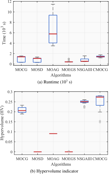
Fig. 5. Performance comparison for different multi-objective algorithms.

To further evaluate the practical performance of each algorithm, Fig. 6 presents the Pareto fronts corresponding to the largest HV values obtained across the 30 independent runs. As illustrated in the figure, the solution sets of certain algorithms, notably MOAG and MOEGS, appear visually sparse. For instance, MOAG seems to have only a single solution, while MOEGS displays approximately seven distinct points. It is important to clarify that this sparsity does not result from a reduction in the number of solutions—since the population size is fixed at 100—but rather from severe clustering of solutions. Specifically, all 100 solutions of MOAG completely overlap at a single point, indicating an extreme lack of diversity. Nevertheless, this converged solution exhibits relatively favorable objective values: a trajectory length of approximately \(9381\) m, a maximum curvature below \(6°/30\) m, and a wellbore stability density around \(1.6\) g/cm\(^3\), suggesting that MOAG maintains acceptable convergence despite its diversity failure.

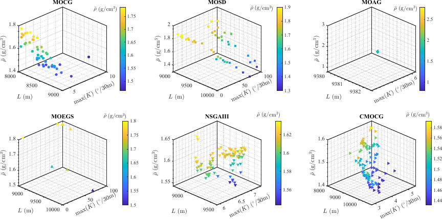
Fig. 6. Comparison of Pareto fronts for multi-objective optimization algorithms.

In contrast, while MOEGS shows slightly better diversity with several clustered solutions, all of them exceed a maximum curvature of \(50°/30\) m—a value that exceeds feasible engineering limits. Such high curvature would likely lead to excessive friction and torque in certain segments of the wellbore, increasing the risk of drilling incidents. Thus, the solutions generated by MOEGS are practically infeasible and represent a planning failure. Similarly, MOSD exhibits greater diversity than MOEGS, but its solutions also consistently surpass the \(50°/30\) m curvature threshold, indicating poor convergence and equally impractical outcomes. Due to these issues—complete loss of diversity in MOAG and severely poor convergence in MOSD and MOEGS—all three algorithms achieve notably low HV values, as reflected in Fig. 5(b).

On the other hand, MOCG, NSGA-III, and CMOCG produce well-distributed Pareto fronts, demonstrating strong diversity and successful trajectory planning. However, differences in convergence are evident, particularly in the second objective (maximum curvature). While solutions from NSGA-III and MOCG generally remain above \(5°/30\) m, CMOCG achieves a subset of solutions with curvature below \(4°/30\) m. This advantage translates into potentially lower friction and torque during drilling, highlighting CMOCG’s superior capability in generating smoother and more practical wellbore trajectories.

5.2.3. Analysis and Discussion

Building upon the results, the comparative performance between gradient-based and gradient-free methods for multi-objective wellbore trajectory planning is analyzed across two dimensions.

1. Gradient-Based Versus Gradient-Free Methods

The computational advantage of gradient-based methods, which is well-established in single-objective optimization ³², was not decisively observed in the multi-objective case. While algorithms like MOAG exhibited significantly higher runtimes than gradient-free counterparts without superior convergence, the proposed CMOCG method only achieved a marginal runtime reduction compared to NSGA-III. This limited performance gain can be attributed to two primary factors. First, the overhead associated with essential multi-objective management mechanisms, such as Pareto ranking and diversity preservation, often dominates the computational cost, diminishing the relative benefit of faster gradient steps. Second, the moderate scale of the presented problem (19 decision variables) remains well-suited for population-based evolutionary algorithms. The potential efficiency of gradient-based methods is likely to become more pronounced in higher-dimensional search spaces, such as those encountered in real-time trajectory optimization for geo-steering, where the number of adjustable parameters is substantially larger. Furthermore, inherent conflicts between competing objectives may increase problem complexity, potentially reducing the effectiveness of local gradient information and thereby limiting speedup.

Regarding solution quality, a key finding is the instability of several gradient-based methods, which exhibited outright planning failures. This contrasts with the robust performance of gradient-free algorithms. The severe loss of solution diversity observed in methods like MOEGS and MOAG points to a fundamental design challenge: without an explicit Pareto-based selection mechanism, gradient directions from multiple objectives can drive the population toward a single, sub-optimal point. The proposed CMOCG method mitigated this issue, maintaining stable performance with high HV (\(> 0.25\)) in most runs.

2. Performance Variation Among Gradient-Based Optimizers

Significant divergence was observed within the category of gradient-based methods themselves, underscoring the critical importance of the core search strategy. The failure of the basic steepest-descent approach (MOSD) highlights its inadequacy for complex, constrained multi-objective landscapes due to non-adaptive step sizes. In contrast, the conjugate gradient strategy employed in MOCG demonstrated markedly better convergence behavior. The CMOCG method builds upon this by integrating specialized mechanisms for diversity preservation and conflict resolution, which collectively enable its solution set to surpass the quality of those from gradient-free methods in key metrics. A detailed ablation study in the following section investigates the contribution of these individual components.

5.3. Ablation Study

To evaluate the effectiveness of the conflict detection and hybrid search strategy modules within the CMOCG algorithm, this study designs four variant algorithms for an ablation study: variant V1 applies the conjugate gradient update only to non-conflicting variables (\(site[j] = 0\)), while conflicting variables (\(site[j] = 1\)) retain their original values; variant V2 applies the conjugate gradient update to all variables, completely disabling the stochastic differential mechanism; variant V3 introduces stochastic differential perturbation only to conflicting variables, leaving non-conflicting variables unchanged; variant V4 employs stochastic differential perturbation for all variables, removing the conjugate gradient update mechanism entirely.

Figure 7 presents the performance comparison results between these variants and the complete CMOCG algorithm. In terms of computation time (Fig. 7(a)), V4 requires the shortest time, while V1 requires the longest. Regarding solution quality (Fig. 7(b)), the normalized hypervolume metrics of both V3 and V4 are close to zero. The HV value of V2 is superior to that of V1, and the complete CMOCG algorithm achieves the highest hypervolume metric.

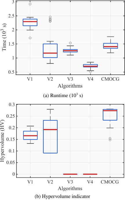
Fig. 7. Ablation study on algorithmic components in CMOCG.

Figure 8 further reveals that the solution sets obtained by V3 and V4 are sparsely distributed and severely deviate from the Pareto front. Although V1 and V2 yield improved results, their solution sets still exhibit deficiencies in both diversity and convergence. In contrast, CMOCG achieves a well-distributed and highly convergent Pareto solution set, validating the efficacy of its hybrid search strategy.

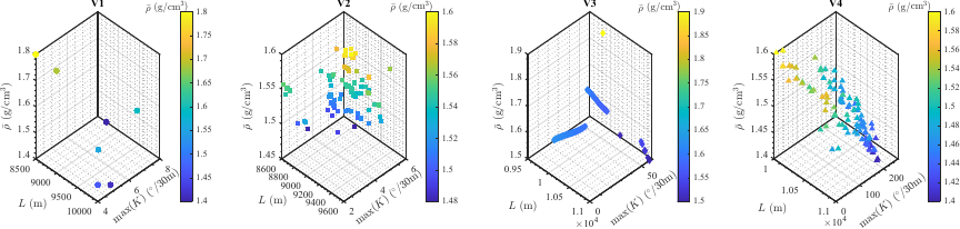
Fig. 8. Comparison of Pareto fronts for ablation study algorithms.

5.4. Analysis of Simulation and Experimental Results for Extended-Reach Wellbore Trajectory

To evaluate the engineering applicability of the wellbore trajectory obtained by the CMOCG algorithm, a solution that achieves a favorable balance among multiple objectives, including friction and torque, total wellbore length, and wellbore stability, was selected from the Pareto front for detailed analysis. Key geometric and engineering parameters of this trajectory are visualized in Fig. 9, which illustrates its spatial profile and the variation of major design parameters with measured depth.

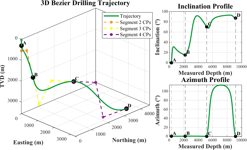
Fig. 9. A simulation result from CMOCG for extended-reach wellbore trajectory.

The trajectory initiates at point A in the vertical section (\(D_A = 299.32~\text{m}\)) and accurately reaches the horizontal target at endpoint D (\(\theta_{inc, D} = 90°\)), with a total measured depth of \(9239.76~\text{m}\). In terms of geometric characteristics, the inclination angle increases smoothly and continuously from \(0°\) at point A to \(16.79°\) at point B, further rising to \(70.32°\) at point C, and finally achieving horizontal drilling at point D. The entire variation process is continuous and smooth without abrupt changes, satisfying \(\mathcal{C}^1\) continuity. The maximum curvature is only \(6.69°/30~\text{m}\), which is well below the operational limits of conventional steering tools, indicating excellent drillability and construction safety. From an engineering perspective, this low curvature value has direct and significant implications for real drilling operations. It ensures that rotary steerable systems can readily execute the trajectory without pushing their planning limits, thereby reducing tool wear and failure risk. More importantly, it directly contributes to lower dogleg severity, which minimizes side forces, reduces friction and torque during drilling and tripping, and enhances overall borehole quality by promoting better cuttings transport.

The azimuth remains highly stable throughout the trajectory, precisely controlled to \(0°\) (true north) at all connection points. Notably, the azimuth deviation at the endpoint D is minimal, still satisfying the target window orientation constraint. The trajectory also demonstrates strong engineering consistency in TVD: the TVD values at points B and C are \(2042.05~\text{m}\) and \(3070.18~\text{m}\), respectively, and the TVD at endpoint D is \(3280.34~\text{m}\), meeting geological objectives. The entire trajectory transitions smoothly in the NED coordinate system, with a reasonable horizontal section extending from point C to D that fulfills the entry requirements of the target window.

In summary, the planned trajectory demonstrates the capability of the CMOCG algorithm to reconcile multi-objective conflicts under complex constraints. While satisfying multiple engineering constraints, including TVD, inclination, azimuth, and curvature limits, the trajectory achieves an effective balance among total length, maximum curvature, and comprehensive wellbore stability (\(\overline{\rho} = 1.61~\mathrm{g/cm}^3\)), exhibiting strong engineering feasibility and overall performance.

To further validate the physical realizability and control performance of the planned trajectory, a hardware-in-the-loop drilling trajectory planning experiment was conducted using the CMOCG algorithm on a dedicated experimental system, as shown in Fig. 10.

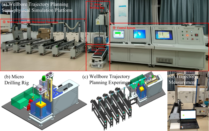
Fig. 10. Semi-physical wellbore trajectory planning experimental system. (a) Overall structure of the experimental platform. The main components include: (1) the micro drilling rig, capable of conducting drilling tests on rock samples in an upright configuration with adjustable penetration rate and rotational speed (mechanical details in (b)); (2) the trajectory-planning mechanical part; (3) an inclinometer housed in a dedicated enclosure for trajectory measurement, where high-precision sensors are inserted into preset pipelines (see (d)) to acquire wellbore trajectory parameters; and (4) the control system comprising a PLC, an industrial computer, and dedicated trajectory-planning software. In the lying posture (c), the rig performs trajectory-related drilling feed operations, working cooperatively with the mechanical part (2) to conduct trajectory-planning experiments.

Considering the physical limitations of the platform, a mapping relationship was established between the actual wellbore trajectory coordinates and the platform coordinates. Let \(P_{real}(N, E, D)\) denote an actual trajectory point and \(P_\mathit{platform}(U, F, R)\) denote the corresponding platform point, where \(F\) represents the longitudinal position of the sliding ring along the drilling direction, \(U\) represents the vertical position, and \(R\) represents the lateral position. The specific mapping is defined as follows:

\begin{equation} \left\{ \begin{aligned} F_k &= \text{fixed position} = [0, 600, 1200, 1800, 2400], \\ U_k &= \dfrac{N_k - N_{\min}}{N_{\max} - N_{\min}} \times U_{\max}, \\ R_k &= \begin{cases} 0, & k = 1, \\ \dfrac{E_k - E_1}{\max\left(\left|E_{2:5} - E_1\right|\right)} \times R_{\max}, & k = 2,3,4,5, \end{cases} \end{aligned} \right. \end{equation}

where the parameters are defined as: the minimum and maximum North coordinates \(N_{\min}\) and \(N_{\max}\), the East coordinate of the wellhead \(E_1\) serving as the reference, the platform’s vertical movement range \(U_{\max} = 500~\mathrm{mm}\), the platform’s lateral movement range \(R_{\max} = 600~\mathrm{mm}\), and the number of sliding rings is 5 with a fixed longitudinal spacing of \(600~\mathrm{mm}\).

Based on the conversion algorithm from actual coordinates \((N, E, D)\) to platform coordinates \((U, R, F)\) as shown in Algorithm 4, the platform positions for the trajectory were calculated. First, the fixed longitudinal positions \(F = [0, 600, 1200, 1800, 2400]\) are initialized, and the normalized parameters \(t_k = F / 2400\) are computed. For each sliding ring \(k\) from 1 to 5, the algorithm finds the point in the original trajectory closest to \(t_k\), calculates the corresponding \((N_k, E_k, D_k)\) coordinates via linear interpolation, and then computes the vertical position \(U_k = ({N_k - N_{\min}})/({N_{\max} - N_{\min}}) \times 500\).

The lateral position \(R\) is computed with special handling: using the wellhead East coordinate \(E_{\text{ref}} = E_1\) as the reference, the sliding ring 1 (wellhead position) is fixed at \(R_1 = 0\) to ensure the wellhead is centered on the platform. For other rings (\(k=2\) to \(5\)), the relative offset \(\Delta E_k = E_k - E_{\text{ref}}\) is calculated. If the maximum offset \(\max(|\Delta E_{2:5}|) > 0\), \(R_k\) is scaled proportionally as \(R_k = {\Delta E_k}/{\max(|\Delta E_{2:5}|)} \times 600\); otherwise, \(R_k = 0\) if all East coordinates are identical. The algorithm finally returns the platform coordinates \((U, F, R)\).

After the trajectory planning module generated the actual trajectory parameters, the coordinate conversion via Algorithm 4 yielded the following platform position coordinates for each sliding ring:

Sliding ring 1: \(F = 0\ \mathrm{mm},\ U = 0.0\ \mathrm{mm},\ R = 0.0\ \mathrm{mm}\)
Sliding ring 2: \(F = 600\ \mathrm{mm},\ U = 7.2\ \mathrm{mm},\ R = 0.0\ \mathrm{mm}\)
Sliding ring 3: \(F = 1200\ \mathrm{mm},\ U = 224.9\ \mathrm{mm},\ R = 0.5\ \mathrm{mm}\)
Sliding ring 4: \(F = 1800\ \mathrm{mm},\ U = 369.3\ \mathrm{mm},\ R = 507.4\ \mathrm{mm}\)
Sliding ring 5: \(F = 2400\ \mathrm{mm},\ U = 453.8\ \mathrm{mm},\ R = 600.0\ \mathrm{mm}\)

The spatial distribution of the sliding rings on the trajectory system is shown in Fig. 11.

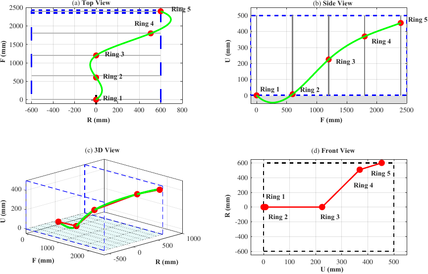
Fig. 11. 3D and multi-view trajectory of the wellbore trajectory planning experimental system.

The servo motors of the trajectory planning system platform were enabled via the PLC communication interface to realize the physical demonstration of the planned trajectory. The actual platform operation is shown in Fig. 12. The experimental results indicate that the drilling trajectory planning platform operates smoothly, and the trajectory planning results generally meet the dynamic performance requirements of the actual system. The trajectory system can largely reproduce the spatial profile of the planned trajectory, with the positions of all sliding rings showing good overall agreement with the theoretical calculations, thereby validating the correctness and feasibility of the proposed CMOCG algorithm and the coordinate mapping relationship. It is also noted that due to factors such as pipe weight and slight errors in motor movement, certain deviations exist between the actual formed trajectory and the simulation results; however, the overall profile remains consistent, reflecting the influence of actual physical conditions on trajectory replication.

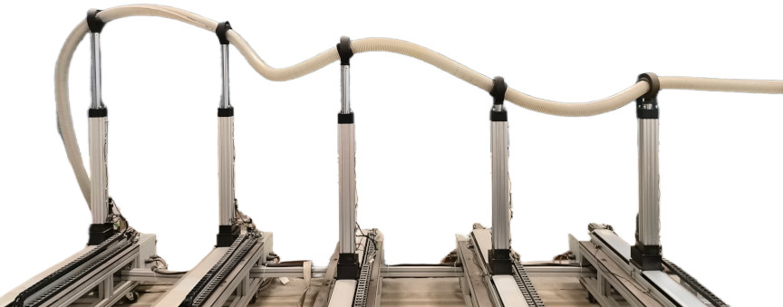
Fig. 12. Side view of the actual trajectory of the wellbore trajectory planning system.

6. Conclusion and Future Outlook

This study addressed the trajectory planning problem for extended-reach horizontal wells by proposing a CMOCG. A multi-objective optimization model was constructed using composite cubic Bézier curves, aiming to minimize the total trajectory length, limit the maximum curvature, and enhance comprehensive wellbore stability, while incorporating critical geometric and engineering constraints.

A major challenge stemmed from the high-dimensional search space resulting from the increased degrees of freedom in multi-segment \(\mathcal{C}^1\)-continuous trajectories—a model with \(m\) segments involves \(6m\) design variables. To tackle this, the CMOCG algorithm incorporates a dual-population cooperative framework that combines finite-difference gradient computation and conjugate gradient-guided local search. Moreover, a conflict identification mechanism coupled with a hybrid differential mutation strategy was introduced to manage gradient conflicts among objectives, thereby improving search capability in highly constrained environments.

Simulation results demonstrated that CMOCG achieves optimal performance with an auxiliary population size of \(N_2 = 10\) and a maximum step adjustment count of \(S_{\max} = 10\). In comparative studies, the proposed algorithm attained the highest normalized hypervolume indicator, outperforming benchmark methods in both convergence and diversity of solutions. Ablation studies confirmed the contribution of the hybrid update strategy to the algorithm’s effectiveness. The selected trajectory satisfied all engineering constraints while successfully balancing wellbore length, curvature control, and wellbore stability indicators.

This research provides an efficient gradient-assisted optimization framework for multi-objective trajectory design in high-dimensional constrained scenarios. Although the proposed method did not exhibit significant computational superiority over traditional multi-objective evolutionary algorithms in the tested five-segment trajectory model—due to its relatively low number of decision variables—it lays the groundwork for more complex applications. According to ³², gradient acceleration techniques in single-objective drilling trajectory optimization can improve computational efficiency by more than 50 times, suggesting substantial potential for acceleration in multi-objective gradient-based methods, particularly in scenarios involving a larger number of segments, such as geological steering drilling that requires real-time trajectory adjustments.

Future work will focus on extending the proposed approach to more complex geological conditions and integrating real-time data for adaptive trajectory updating. It is anticipated that the computational advantages of gradient-based optimization will become more pronounced in these high-dimensional settings. On the other hand, handling multi-objective constraints remains more challenging than in single-objective optimization, and the presence of multi-objective gradient conflicts further impedes computational efficiency. Therefore, further research into improving the mechanisms of multi-objective gradient algorithms, especially regarding constraint handling and conflict resolution, constitutes a promising direction for future work.

Appendix A. Wellbore Trajectory Planning Using Bézier Curves

Bézier curves can be defined using Bernstein basis functions as shown in Eq. \(\eqref{eq:Bensteins}\):

\begin{equation} \label{eq:Bensteins} B_{i,n}(s) = \binom{n}{i} s^{i} (1 - s)^{n-i}, \quad i = 0,\dots,n; \; s \in [0, 1], \end{equation}

where \(\begin{pmatrix}\scriptstyle n\\ \scriptstyle i \end{pmatrix}\) denotes the binomial coefficient. Given a set of \(n+1\) control points \(P_0, P_1, \dots, P_n\), the \(n\)-th degree Bézier curve \(C_n\) is obtained by the weighted blending of these control points using the basis functions:

\begin{align} C_n(s) &= \displaystyle\sum\limits_{i=0}^{n} B_{i,n}(s) \cdot P_i \nonumber \\ &= \displaystyle\sum\limits_{i=0}^{n} \left[ \binom{n}{i} s^{i} (1-s)^{n-i} \right] P_i, \quad s \in [0,1]. \label{eq:bezier} \end{align}

In wellbore trajectory planning, a second-degree Bézier curve cannot independently control the directions at its endpoints; Bézier curves of fourth-degree or higher are prone to non-physical oscillations, making it difficult to generate smooth trajectories. In contrast, the third-degree Bézier curve provides natural curvature variation, avoiding abrupt stress changes on the drill string, thereby reducing wear and making it an ideal choice for modeling wellbore trajectories.

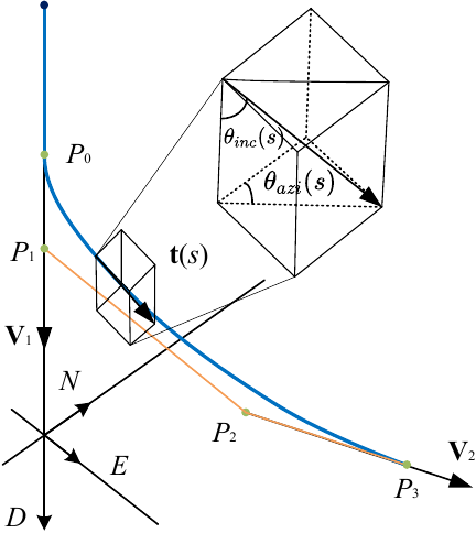
Fig. 13. Computational model of a wellbore trajectory using a third-degree Bézier curve.

As shown in Fig. 13, the coordinates of a trajectory survey point \([N(s), E(s), D(s)]^\top\) on the third-degree Bézier curve model can be calculated by the parametric function \(C(s)\) with respect to \(s\):

\begin{equation} C(s) = (1 - s)^3 \cdot P_0 + 3 \cdot (1 - s)^2 \cdot s \cdot P_1 + 3 \cdot (1 - s) \cdot s^2 \cdot P_2 + s^3 \cdot P_3, \label{eq:beziereq} \end{equation}

where \(P_0\), \(P_1\), \(P_2\), and \(P_3\) are the control points of the third-degree Bézier curve trajectory model. \(P_0\) and \(P_3\) are also the starting point and target point of the wellbore trajectory, respectively. \(P_1\) and \(P_2\) are related to the direction vector \(\mathbf{v}_1\) at the starting point and the direction vector \(\mathbf{v}_2\) at the target point, i.e.:

\begin{equation} P_1 = P_0 + d_1 \cdot \mathbf{v}_1, \quad P_2 = P_3 - d_2 \cdot \mathbf{v}_2, \end{equation}

\(d_1\) and \(d_2\) are control parameters adjusting the distances of \(P_1\) and \(P_2\) from the starting point and target point, respectively. \(\mathbf{v}_1\) and \(\mathbf{v}_2\) can be expressed using the inclination angle \(\theta_{inc,1}\) and azimuth angle \(\theta_{azi,1}\) at the starting point, and the inclination angle \(\theta_{inc,n}\) and azimuth angle \(\theta_{azi,n}\) at the target point:

\begin{equation} \begin{cases} \mathbf{v}_1 = [\cos \theta_{inc,1} , \sin \theta_{inc,1} \cos \theta_{azi,1}, \sin \theta_{inc,1} \sin \theta_{azi,1}]^\top, \\ \mathbf{v}_2 = [\cos \theta_{inc,n} , \sin \theta_{inc,n} \cos \theta_{azi,n}, \sin \theta_{inc,n} \sin \theta_{azi,n}]^\top. \end{cases} \end{equation}

The inclination and azimuth angles along the Bézier curve can be obtained by calculating the tangent vector \(\mathbf{t}(s)\) of the curve at that point, as shown in Fig. 13. The first derivative of the curve \(C(s)\) with respect to the parameter \(s\) gives the tangent vector:

\begin{align} \mathbf{t}(s) = \frac{dC(s)}{ds} &= -3(1-s)^2 P_0 + 3\left(1 - 4s + 3s^2\right) P_1 \nonumber \\ &\phantom{=~} + 3\left(2s - 3s^2\right) P_2 + 3s^2 P_3. \label{eq:tangent_vector} \end{align}

The inclination angle is defined as the angle between the tangent vector \(\mathbf{t}(s)\) and the direction of increasing vertical depth. Let \(\mathbf{t}(s) = [t_N(s), t_E(s), t_D(s)]^\top\), then:

\begin{equation} \label{eq:inclination} \theta_{inc}(s) = \cos^{-1} \left( \frac{t_D(s)}{\|\mathbf{t}(s)\|} \right), \end{equation}

where \(\|\mathbf{t}(s)\|=\sqrt{t_N^2(s)+t_E^2(s)+t_D^2(s)}\) is the magnitude of the tangent vector. The azimuth angle is the angle between the projection of the tangent vector \(\mathbf{t}(s)\) onto the NE horizontal plane and the true north direction:

\begin{equation} \label{eq:azimuth} \theta_{azi}(s) = \arctan2\left(t_E(s), t_N(s)\right). \end{equation}

A composite Bézier curve \(\mathbb{C}\) can be represented as the union of multiple piecewise Bézier curves, i.e., \(\mathbb{C} = \bigcup_{i=1}^{m} C_i(s)\). Fig. 14 shows an example of the connection of two cubic Bézier curves. The first blue curve \(C_1(s)\) has endpoints A and B, with direction vectors \(a\) and \(b\), respectively. The second orange curve \(C_2(s)\) has endpoints B and C, with direction vectors \(b\) and \(c\), respectively. Clearly, the coincidence at point B ensures \(\mathcal{C}^0\) continuity of the entire trajectory. Control points \(P_{a1}\) and \(P_{b1}\) control the shape of \(C_1(s)\), while \(P_{b2}\) and \(P_{c2}\) control the shape of \(C_2(s)\).

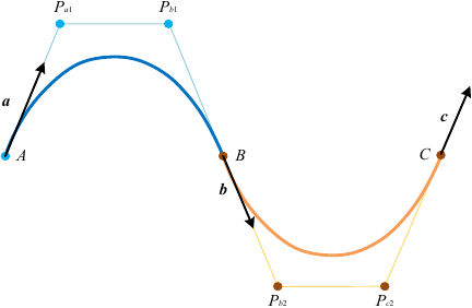
Fig. 14. Composite curve model of two third-degree Bézier curves.

From Eq. \(\eqref{eq:beziereq}\), the expressions for \(C_1(s)\) and \(C_2(s)\) are:

\begin{equation} \begin{cases} \begin{aligned} C_1(s) &= (1-s)^3 A + 3(1-s)^2 s P_{a1} \\ &\quad + 3(1-s) s^2 P_{b1} + s^3 B, \\ C_2(s) &= (1-s)^3 B + 3(1-s)^2 s P_{b2} \\ &\quad + 3(1-s) s^2 P_{c2} + s^3 C. \end{aligned} \end{cases} \label{eq:c0eq} \end{equation}

Computing the first derivatives yields:

\begin{equation} \begin{cases} \begin{aligned} C_1'(s) &= -3(1-s)^2 A + 3\left(1 - 4s + 3s^2\right) P_{a1} \\ &\quad + 3\left(2s - 3s^2\right) P_{b1} + 3s^2 B, \\ C_2'(s) &= -3(1-s)^2 B + 3\left(1 - 4s + 3s^2\right) P_{b2} \\ &\quad + 3\left(2s - 3s^2\right) P_{c2} + 3s^2 C. \end{aligned} \end{cases} \label{eq:c1c2_prime} \end{equation}

Computing the second derivatives yields:

\begin{equation} \begin{cases} \begin{aligned} C_1''(s) &= 6(1-s) A + 3(-4 + 6s) P_{a1} \\ &\quad + 3(2 - 6s) P_{b1} + 6s B, \\ C_2''(s) &= 6(1-s) B + 3(-4 + 6s) P_{b2} \\ &\quad + 3(2 - 6s) P_{c2} + 6s C. \end{aligned} \end{cases} \end{equation}

The conditions for \(\mathcal{C}^1\) and \(\mathcal{C}^2\) continuity at point B between \(C_1(s)\) and \(C_2(s)\) can be directly derived. For \(\mathcal{C}^1\) continuity:

\begin{align} C_1'(s=1) &= -3P_{b1} + 3B \nonumber \\ &= -3B + 3P_{b2} = C_2'(s=0), \end{align}

i.e.,

\begin{equation} 2B = P_{b1} + P_{b2}. \label{eq:EqC1continuity} \end{equation}

Therefore, for a composite Bézier curve to achieve \(\mathcal{C}^1\) continuity, the distance from the control point of the previous segment to the connection point must equal the distance from the connection point to the control point of the next segment. For \(\mathcal{C}^2\) continuity:

\begin{align} C_1''(s=1) &= 6P_{a1} - 12P_{b1} + 6B \nonumber \\ &= 6B - 12P_{b2} + 6P_{c2} = C_2''(s=0), \end{align}

i.e.,

\begin{equation} P_{a1}-2P_{b1} = P_{c2} -2P_{b2}. \end{equation}

Acknowledgments

This work was supported by the National Natural Science Foundation of China [Grant Number 62333019]; the China Postdoctoral Science Foundation [Grant Numbers 2023TQ0337 and 2024M763061]; Fundamental Research Funds for the Central Universities, China University of Geosciences (Wuhan); 111 Project [Grant Number B17040].

References

[1] D. Zhang, M. Wu, C. Lu, L. Chen, W. Cao, and J. Hu, “Intelligent Compensating Method for MPC-Based Deviation Correction with Stratum Uncertainty in Vertical Drilling Process,” J. Adv. Comput. Intell. Inform., Vol.25, No.1, pp. 23-30, 2021. https://doi.org/10.20965/jaciii.2021.p0023
[2] H. Wei, N. Yao, H. Tian, Y. Yao, J. Zhang, and H. Li, “A Predicting Model for Near-Horizontal Directional Drilling Path Based on BP Neural Network in Underground Coal Mine,” J. Adv. Comput. Intell. Inform., Vol.26, No.3, pp. 279-288, 2022. https://doi.org/10.20965/jaciii.2022.p0279
[3] W. Li, M. Wu, S. Chen, L. Mu, C. Lu, and L. Chen, “Design of an Intelligent Control System for Compound Directional Drilling in Underground Coal Mines,” J. Adv. Comput. Intell. Inform., Vol.28, No.4, pp. 1052-1062, 2024. https://doi.org/10.20965/jaciii.2024.p1052
[4] D. Chen, K. Mao, Z. Ye, W. Li, W. Yan, and H. Wang, “An artificial intelligent well trajectory design method combining both geological and engineering objectives,” Geoenergy Sci. Eng., Vol.236, Article No.212736, 2024. https://doi.org/10.1016/j.geoen.2024.212736
[5] Z. Cai, X. Lai, M. Wu, C. Lu, and L. Chen, “Trajectory Azimuth Control Based on Equivalent Input Disturbance Approach for Directional Drilling Process,” J. Adv. Comput. Intell. Inform., Vol.25, No.1, pp. 31-39, 2021. https://doi.org/10.20965/jaciii.2021.p0031
[6] Z. Cai and G. Hu, “Stability Analysis of Drilling Inclination System with Time-Varying Delay via Free-Matrix-Based Lyapunov–Krasovskii Functional,” J. Adv. Comput. Intell. Inform., Vol.25, No.6, pp. 1031-1038, 2021. https://doi.org/10.20965/jaciii.2021.p1031
[7] S. Vlemmix, G. J. P. Joosten, D. R. Brouwer, and J. D. Jansen, “Adjoint-Based Well Trajectory Optimization in a Thin Oil Rim,” EUROPEC/EAGE Conf. and Exhib. (09EURO), Article No.SPE-121891-MS, 2009. https://doi.org/10.2118/121891-MS
[8] R. G. Hanea, P. Casanova, F. H. Wilschut, and R. M. Fonseca, “Well Trajectory Optimization Constrained to Structural Uncertainties,” SPE Res. Simul. Conf., Article No.SPE-182680-MS, 2017. https://doi.org/10.2118/182680-MS
[9] E. G. D. Barros, A. Chitu, and O. Leeuwenburgh, “Ensemble-based well trajectory and drilling schedule optimization-application to the Olympus benchmark model,” Comput. Geosci., Vol.24, No.6, pp. 2095-2109, 2020. https://doi.org/10.1007/s10596-020-09952-7
[10] X. Wu and K. Zhang, “Three-dimensional trajectory design for horizontal well based on optimal switching algorithms,” ISA Trans., Vol.58, pp. 348-356, 2015. https://doi.org/10.1016/j.isatra.2015.04.002
[11] Y. Guo and E. Feng, “Nonlinear dynamical systems of trajectory design for 3D horizontal well and their optimal controls,” J. Comput. Appl. Math., Vol.212, Issue 2, pp. 179-186, 2008. https://doi.org/10.1016/j.cam.2006.11.034
[12] R. Lu and A. C. Reynolds, “Joint Optimization of Well Locations, Types, Drilling Order, and Controls Given a Set of Potential Drilling Paths,” SPE J., Vol.25, Issue 03, pp. 1285-1306, 2020. https://doi.org/10.2118/193885-PA
[13] U. Singh, R. Pathan, A. D. Joshi, A. Cavé, C. Fouchard, and A. Baume, “Accelerated Design of Sidetrack and Deepening Well Trajectories,” SPE J., Vol.29, Issue 04, pp. 1862-1872, 2024. https://doi.org/10.2118/218395-PA
[14] W. Li, X. Yang, C. Lu, Q. Li, P. Fang, X. Wu, H. Huang, H. Fan, N. Yao, H. Tian, and M. Wu, “Modeling and optimization of trajectory deviation for compound directional drilling in coal mines,” Neurocomputing, Vol.618, Article No.129029, 2025. https://doi.org/10.1016/j.neucom.2024.129029
[15] J. Shu, G. Han, Z. Yue, L. Cheng, Y. Dong, and X. Liang, “Optimizing Well Trajectories for Enhanced Oil Production in Naturally Fractured Reservoirs: Integrating Particle Swarm Optimization with an Innovative Semi-Analytical Model Framework,” SPE J., Vol.30, Issue 02, pp. 957-975, 2025. https://doi.org/10.2118/223939-PA
[16] Z. Wang, D. Gao, and J. Liu, “Multi-objective sidetracking horizontal well trajectory optimization in cluster wells based on DS algorithm,” J. Petrol. Sci. Eng., Vol.147, pp. 771-778, 2016. https://doi.org/10.1016/j.petrol.2016.09.046
[17] R. Khosravanian, V. Mansouri, D. A. Wood, and M. R. Alipour, “A comparative study of several metaheuristic algorithms for optimizing complex 3-D well-path designs,” J. Pet. Explor. Prod. Technol., Vol.8, No.4, pp. 1487-1503, 2018. https://doi.org/10.1007/s13202-018-0447-2
[18] J. Xu and X. Chen, “Bat Algorithm Optimizer for Drilling Trajectory Designing under Wellbore Stability Constraints,” 2018 37th Chinese Control Conf. (CCC), pp. 10276-10280, 2018. https://doi.org/10.23919/ChiCC.2018.8483403
[19] K. Biswas, M. T. Rahman, A. H. Almulihi, F. Alassery, M. A. H. Al Askary, T. B. Hai, S. S. Kabir, A. I. Khan, and R. Ahmed, “Uncertainty handling in wellbore trajectory design: A modified cellular spotted hyena optimizer-based approach,” J. Pet. Explor. Prod. Technol., Vol.12, pp. 2643-2661, 2022. https://doi.org/10.1007/s13202-022-01458-5
[20] S. Sun, Y. Gao, X. Sun, J. Wu, and H. Chang, “Intelligent optimization of horizontal wellbore trajectory based on reinforcement learning,” Geoenergy Sci. Eng., Vol.244, Article No.213479, 2025. https://doi.org/10.1016/j.geoen.2024.213479
[21] W. Zhu, Y. Liu, L. Wang, J. Cao, Y. Li, and Y. Ma, “Deep Reinforcement Learning for Well Trajectory Design with Collision Avoidance,” SPE J., Vol.30, Issue 08, pp. 4545-4560, 2025. https://doi.org/10.2118/228295-PA
[22] S. Ghadami, H. Biglarian, H. Beyrami, and M. Salimi, “Optimization of multilateral well trajectories using pattern search and genetic algorithms,” Results Eng., Vol.16, Article No.100722, 2022. https://doi.org/10.1016/j.rineng.2022.100722
[23] A. Lamghari, “Mine Planning and Oil Field Development: A Survey and Research Potentials,” Math. Geosci., Vol.49, No.3, pp. 395-437, 2017. https://doi.org/10.1007/s11004-017-9676-z
[24] W. Huang, M. Wu, L. Chen, X. Chen, and W. Cao, “Multi-objective drilling trajectory optimization using decomposition method with minimum fuzzy entropy-based comprehensive evaluation,” Appl. Soft Comput., Vol.107, Article No.107392, 2021. https://doi.org/10.1016/j.asoc.2021.107392
[25] W. Huang, M. Wu, L. Chen, J. She, H. Hashimoto, and S. Kawata, “Multiobjective Drilling Trajectory Optimization Considering Parameter Uncertainties,” IEEE Trans. on Systems, Man, and Cybernetics: Systems, Vol.52, Issue 2, pp. 1224-1233, 2022. https://doi.org/10.1109/TSMC.2020.3019428
[26] J. Xu, X. Chen, W. Cao, and M. Wu, “Multi-objective trajectory planning in the multiple strata drilling process: A bi-directional constrained co-evolutionary optimizer with Pareto front learning,” Expert Syst. Appl., Vol.238, Part F, Article No.122119, 2024. https://doi.org/10.1016/j.eswa.2023.122119
[27] Z. Wang, S.-L. Shen, D. Chen, W. Li, W. Li, and Z. Fan, “Multi-objective optimization of the wellbore trajectory considering both geological and engineering factors,” Geoenergy Sci. Eng., Vol.246, Article No.213647, 2025. https://doi.org/10.1016/j.geoen.2025.213647
[28] J. Xu, X. Chen, Y. Zhou, M. Zhang, W. Cao, and M. Wu, “Expensive deviation-correction drilling trajectory planning: A constrained multi-objective Bayesian optimization with feasibility-oriented bi-objective acquisition function,” Control Eng. Pract., Vol.156, Article No.106240, 2025. https://doi.org/10.1016/j.conengprac.2025.106240
[29] H. Yavari, J. Qajar, B. S. Aadnoy, and R. Khosravanian, “Selection of Optimal Well Trajectory Using Multi-Objective Genetic Algorithm and TOPSIS Method,” Arab. J. Sci. Eng., Vol.48, No.12, pp. 16831-16855, 2023. https://doi.org/10.1007/s13369-023-08149-1
[30] J. Kudela, “A critical problem in benchmarking and analysis of evolutionary computation methods,” Nat. Mach. Intell., Vol.4, No.12, pp. 1238-1245, 2022. https://doi.org/10.1038/s42256-022-00579-0
[31] K.-Z. Liu and C. Gan, “Deterministic Gradient-Descent Learning of Linear Regressions: Adaptive Algorithms, Convergence Analysis and Noise Compensation,” IEEE Trans. Pattern Anal. Mach. Intell., Vol.46, Issue 12, pp. 7867-7877, 2024. https://doi.org/10.1109/TPAMI.2024.3399312
[32] D. A. Wood, “Constrained optimization assists deviated wellbore trajectory selection from families of quadratic and cubic Bezier curves,” Gas Sci. Eng., Vol.110, Article No.204869, 2023. https://doi.org/10.1016/j.jgsce.2022.204869
[33] E. M. E. M. Shokir, M. K. Emera, S. M. Eid, and A. W. Wally, “A New Optimization Model for 3D Well Design,” Oil and Gas Sci. Technol., Vol.59, No.3, pp. 255-266, 2004. https://doi.org/10.2516/ogst:2004018
[34] J. Fliege and B. F. Svaiter, “Steepest descent methods for multicriteria optimization,” Math. Methods Oper. Res., Vol.51, No.3, pp. 479-494, 2000. https://doi.org/10.1007/s001860000043
[35] X. Liu and A. C. Reynolds, “A multiobjective steepest descent method with applications to optimal well control,” Comput. Geosci., Vol.20, No.2, pp. 355-374, 2016. https://doi.org/10.1007/s10596-016-9562-7
[36] K. Izui, T. Yamada, S. Nishiwaki, and K. Tanaka, “Multiobjective optimization using an aggregative gradient-based method,” Struct. Multidiscip. Optim., Vol.51, No.1, pp. 173-182, 2015. https://doi.org/10.1007/s00158-014-1125-8
[37] C. K. Goh, Y. S. Ong, K. C. Tan, and E. J. Teoh, “An investigation on evolutionary gradient search for multi-objective optimization,” 2008 IEEE Congress on Evolutionary Computation (IEEE World Congress on Computational Intelligence), pp. 3741-3746, 2008. https://doi.org/10.1109/CEC.2008.4631304
[38] K. Deb and H. Jain, “An Evolutionary Many-Objective Optimization Algorithm Using Reference-Point-Based Nondominated Sorting Approach, Part I: Solving Problems with Box Constraints,” IEEE Trans. Evol. Comput., Vol.18, Issue 4, pp. 577-601, 2014. https://doi.org/10.1109/TEVC.2013.2281535
[39] Y. Tian, R. Cheng, X. Zhang, and Y. Jin, “PlatEMO: A MATLAB Platform for Evolutionary Multi-Objective Optimization,” IEEE Comput. Intell. Mag., Vol.12, Issue 4, pp. 73-87, 2017. https://doi.org/10.1109/MCI.2017.2742868

This article is published under a Creative Commons Attribution-NoDerivatives 4.0 Internationa License.

[B1] [1] D. Zhang, M. Wu, C. Lu, L. Chen, W. Cao, and J. Hu, “Intelligent Compensating Method for MPC-Based Deviation Correction with Stratum Uncertainty in Vertical Drilling Process,” J. Adv. Comput. Intell. Inform., Vol.25, No.1, pp. 23-30, 2021. https://doi.org/10.20965/jaciii.2021.p0023

[B2] [2] H. Wei, N. Yao, H. Tian, Y. Yao, J. Zhang, and H. Li, “A Predicting Model for Near-Horizontal Directional Drilling Path Based on BP Neural Network in Underground Coal Mine,” J. Adv. Comput. Intell. Inform., Vol.26, No.3, pp. 279-288, 2022. https://doi.org/10.20965/jaciii.2022.p0279

[B3] [3] W. Li, M. Wu, S. Chen, L. Mu, C. Lu, and L. Chen, “Design of an Intelligent Control System for Compound Directional Drilling in Underground Coal Mines,” J. Adv. Comput. Intell. Inform., Vol.28, No.4, pp. 1052-1062, 2024. https://doi.org/10.20965/jaciii.2024.p1052

[B4] [4] D. Chen, K. Mao, Z. Ye, W. Li, W. Yan, and H. Wang, “An artificial intelligent well trajectory design method combining both geological and engineering objectives,” Geoenergy Sci. Eng., Vol.236, Article No.212736, 2024. https://doi.org/10.1016/j.geoen.2024.212736

[B5] [5] Z. Cai, X. Lai, M. Wu, C. Lu, and L. Chen, “Trajectory Azimuth Control Based on Equivalent Input Disturbance Approach for Directional Drilling Process,” J. Adv. Comput. Intell. Inform., Vol.25, No.1, pp. 31-39, 2021. https://doi.org/10.20965/jaciii.2021.p0031

[B6] [6] Z. Cai and G. Hu, “Stability Analysis of Drilling Inclination System with Time-Varying Delay via Free-Matrix-Based Lyapunov–Krasovskii Functional,” J. Adv. Comput. Intell. Inform., Vol.25, No.6, pp. 1031-1038, 2021. https://doi.org/10.20965/jaciii.2021.p1031

[B7] [7] S. Vlemmix, G. J. P. Joosten, D. R. Brouwer, and J. D. Jansen, “Adjoint-Based Well Trajectory Optimization in a Thin Oil Rim,” EUROPEC/EAGE Conf. and Exhib. (09EURO), Article No.SPE-121891-MS, 2009. https://doi.org/10.2118/121891-MS

[B8] [8] R. G. Hanea, P. Casanova, F. H. Wilschut, and R. M. Fonseca, “Well Trajectory Optimization Constrained to Structural Uncertainties,” SPE Res. Simul. Conf., Article No.SPE-182680-MS, 2017. https://doi.org/10.2118/182680-MS

[B9] [9] E. G. D. Barros, A. Chitu, and O. Leeuwenburgh, “Ensemble-based well trajectory and drilling schedule optimization-application to the Olympus benchmark model,” Comput. Geosci., Vol.24, No.6, pp. 2095-2109, 2020. https://doi.org/10.1007/s10596-020-09952-7

[B10] [10] X. Wu and K. Zhang, “Three-dimensional trajectory design for horizontal well based on optimal switching algorithms,” ISA Trans., Vol.58, pp. 348-356, 2015. https://doi.org/10.1016/j.isatra.2015.04.002

[B11] [11] Y. Guo and E. Feng, “Nonlinear dynamical systems of trajectory design for 3D horizontal well and their optimal controls,” J. Comput. Appl. Math., Vol.212, Issue 2, pp. 179-186, 2008. https://doi.org/10.1016/j.cam.2006.11.034

[B12] [12] R. Lu and A. C. Reynolds, “Joint Optimization of Well Locations, Types, Drilling Order, and Controls Given a Set of Potential Drilling Paths,” SPE J., Vol.25, Issue 03, pp. 1285-1306, 2020. https://doi.org/10.2118/193885-PA

[B13] [13] U. Singh, R. Pathan, A. D. Joshi, A. Cavé, C. Fouchard, and A. Baume, “Accelerated Design of Sidetrack and Deepening Well Trajectories,” SPE J., Vol.29, Issue 04, pp. 1862-1872, 2024. https://doi.org/10.2118/218395-PA

[B14] [14] W. Li, X. Yang, C. Lu, Q. Li, P. Fang, X. Wu, H. Huang, H. Fan, N. Yao, H. Tian, and M. Wu, “Modeling and optimization of trajectory deviation for compound directional drilling in coal mines,” Neurocomputing, Vol.618, Article No.129029, 2025. https://doi.org/10.1016/j.neucom.2024.129029

[B15] [15] J. Shu, G. Han, Z. Yue, L. Cheng, Y. Dong, and X. Liang, “Optimizing Well Trajectories for Enhanced Oil Production in Naturally Fractured Reservoirs: Integrating Particle Swarm Optimization with an Innovative Semi-Analytical Model Framework,” SPE J., Vol.30, Issue 02, pp. 957-975, 2025. https://doi.org/10.2118/223939-PA

[B16] [16] Z. Wang, D. Gao, and J. Liu, “Multi-objective sidetracking horizontal well trajectory optimization in cluster wells based on DS algorithm,” J. Petrol. Sci. Eng., Vol.147, pp. 771-778, 2016. https://doi.org/10.1016/j.petrol.2016.09.046

[B17] [17] R. Khosravanian, V. Mansouri, D. A. Wood, and M. R. Alipour, “A comparative study of several metaheuristic algorithms for optimizing complex 3-D well-path designs,” J. Pet. Explor. Prod. Technol., Vol.8, No.4, pp. 1487-1503, 2018. https://doi.org/10.1007/s13202-018-0447-2

[B18] [18] J. Xu and X. Chen, “Bat Algorithm Optimizer for Drilling Trajectory Designing under Wellbore Stability Constraints,” 2018 37th Chinese Control Conf. (CCC), pp. 10276-10280, 2018. https://doi.org/10.23919/ChiCC.2018.8483403

[B19] [19] K. Biswas, M. T. Rahman, A. H. Almulihi, F. Alassery, M. A. H. Al Askary, T. B. Hai, S. S. Kabir, A. I. Khan, and R. Ahmed, “Uncertainty handling in wellbore trajectory design: A modified cellular spotted hyena optimizer-based approach,” J. Pet. Explor. Prod. Technol., Vol.12, pp. 2643-2661, 2022. https://doi.org/10.1007/s13202-022-01458-5

[B20] [20] S. Sun, Y. Gao, X. Sun, J. Wu, and H. Chang, “Intelligent optimization of horizontal wellbore trajectory based on reinforcement learning,” Geoenergy Sci. Eng., Vol.244, Article No.213479, 2025. https://doi.org/10.1016/j.geoen.2024.213479

[B21] [21] W. Zhu, Y. Liu, L. Wang, J. Cao, Y. Li, and Y. Ma, “Deep Reinforcement Learning for Well Trajectory Design with Collision Avoidance,” SPE J., Vol.30, Issue 08, pp. 4545-4560, 2025. https://doi.org/10.2118/228295-PA

[B22] [22] S. Ghadami, H. Biglarian, H. Beyrami, and M. Salimi, “Optimization of multilateral well trajectories using pattern search and genetic algorithms,” Results Eng., Vol.16, Article No.100722, 2022. https://doi.org/10.1016/j.rineng.2022.100722

[B23] [23] A. Lamghari, “Mine Planning and Oil Field Development: A Survey and Research Potentials,” Math. Geosci., Vol.49, No.3, pp. 395-437, 2017. https://doi.org/10.1007/s11004-017-9676-z

[B24] [24] W. Huang, M. Wu, L. Chen, X. Chen, and W. Cao, “Multi-objective drilling trajectory optimization using decomposition method with minimum fuzzy entropy-based comprehensive evaluation,” Appl. Soft Comput., Vol.107, Article No.107392, 2021. https://doi.org/10.1016/j.asoc.2021.107392

[B25] [25] W. Huang, M. Wu, L. Chen, J. She, H. Hashimoto, and S. Kawata, “Multiobjective Drilling Trajectory Optimization Considering Parameter Uncertainties,” IEEE Trans. on Systems, Man, and Cybernetics: Systems, Vol.52, Issue 2, pp. 1224-1233, 2022. https://doi.org/10.1109/TSMC.2020.3019428

[B26] [26] J. Xu, X. Chen, W. Cao, and M. Wu, “Multi-objective trajectory planning in the multiple strata drilling process: A bi-directional constrained co-evolutionary optimizer with Pareto front learning,” Expert Syst. Appl., Vol.238, Part F, Article No.122119, 2024. https://doi.org/10.1016/j.eswa.2023.122119

[B27] [27] Z. Wang, S.-L. Shen, D. Chen, W. Li, W. Li, and Z. Fan, “Multi-objective optimization of the wellbore trajectory considering both geological and engineering factors,” Geoenergy Sci. Eng., Vol.246, Article No.213647, 2025. https://doi.org/10.1016/j.geoen.2025.213647

[B28] [28] J. Xu, X. Chen, Y. Zhou, M. Zhang, W. Cao, and M. Wu, “Expensive deviation-correction drilling trajectory planning: A constrained multi-objective Bayesian optimization with feasibility-oriented bi-objective acquisition function,” Control Eng. Pract., Vol.156, Article No.106240, 2025. https://doi.org/10.1016/j.conengprac.2025.106240

[B29] [29] H. Yavari, J. Qajar, B. S. Aadnoy, and R. Khosravanian, “Selection of Optimal Well Trajectory Using Multi-Objective Genetic Algorithm and TOPSIS Method,” Arab. J. Sci. Eng., Vol.48, No.12, pp. 16831-16855, 2023. https://doi.org/10.1007/s13369-023-08149-1

[B30] [30] J. Kudela, “A critical problem in benchmarking and analysis of evolutionary computation methods,” Nat. Mach. Intell., Vol.4, No.12, pp. 1238-1245, 2022. https://doi.org/10.1038/s42256-022-00579-0

[B31] [31] K.-Z. Liu and C. Gan, “Deterministic Gradient-Descent Learning of Linear Regressions: Adaptive Algorithms, Convergence Analysis and Noise Compensation,” IEEE Trans. Pattern Anal. Mach. Intell., Vol.46, Issue 12, pp. 7867-7877, 2024. https://doi.org/10.1109/TPAMI.2024.3399312

[B32] [32] D. A. Wood, “Constrained optimization assists deviated wellbore trajectory selection from families of quadratic and cubic Bezier curves,” Gas Sci. Eng., Vol.110, Article No.204869, 2023. https://doi.org/10.1016/j.jgsce.2022.204869

[B33] [33] E. M. E. M. Shokir, M. K. Emera, S. M. Eid, and A. W. Wally, “A New Optimization Model for 3D Well Design,” Oil and Gas Sci. Technol., Vol.59, No.3, pp. 255-266, 2004. https://doi.org/10.2516/ogst:2004018

[B34] [34] J. Fliege and B. F. Svaiter, “Steepest descent methods for multicriteria optimization,” Math. Methods Oper. Res., Vol.51, No.3, pp. 479-494, 2000. https://doi.org/10.1007/s001860000043

[B35] [35] X. Liu and A. C. Reynolds, “A multiobjective steepest descent method with applications to optimal well control,” Comput. Geosci., Vol.20, No.2, pp. 355-374, 2016. https://doi.org/10.1007/s10596-016-9562-7

[B36] [36] K. Izui, T. Yamada, S. Nishiwaki, and K. Tanaka, “Multiobjective optimization using an aggregative gradient-based method,” Struct. Multidiscip. Optim., Vol.51, No.1, pp. 173-182, 2015. https://doi.org/10.1007/s00158-014-1125-8

[B37] [37] C. K. Goh, Y. S. Ong, K. C. Tan, and E. J. Teoh, “An investigation on evolutionary gradient search for multi-objective optimization,” 2008 IEEE Congress on Evolutionary Computation (IEEE World Congress on Computational Intelligence), pp. 3741-3746, 2008. https://doi.org/10.1109/CEC.2008.4631304

[B38] [38] K. Deb and H. Jain, “An Evolutionary Many-Objective Optimization Algorithm Using Reference-Point-Based Nondominated Sorting Approach, Part I: Solving Problems with Box Constraints,” IEEE Trans. Evol. Comput., Vol.18, Issue 4, pp. 577-601, 2014. https://doi.org/10.1109/TEVC.2013.2281535

[B39] [39] Y. Tian, R. Cheng, X. Zhang, and Y. Jin, “PlatEMO: A MATLAB Platform for Evolutionary Multi-Objective Optimization,” IEEE Comput. Intell. Mag., Vol.12, Issue 4, pp. 73-87, 2017. https://doi.org/10.1109/MCI.2017.2742868

A Conjugate Gradient-Accelerated Constrained Multi-Objective Optimizer for High-Dimensional Problems with Application to Wellbore Trajectory Planning

Jiafeng Xu*1,*2,*3 , Xin Chen*1,*2,*3,*4,† , and Yang Zhou*1,*2,*3

1. Introduction

2. Multi-Objective Wellbore Trajectory Planning in Multiple Strata

2.1. Conventional Geometric Indicators of Wellbore Trajectory Planning

2.2. Formation-Related Indicators for Wellbore Trajectory

3. Medium-to-High Dimensional Composite Wellbore Trajectory Planning

3.1. Degrees of Freedom in Composite Cubic Bézier Curve Trajectory Modeling

3.2. Extended-Reach Horizontal Wellbore Trajectory Planning

4. Constrained Multi-Objective Optimization with Conjugate Gradient

4.1. Dual-Population Optimization Framework with Conjugate Gradient Assisted Search

4.2. Finite Difference Approximation for Gradient Calculation

4.3. Hybrid Search with Adaptive Step Size for Conflict Handling

5. Experiments

5.1. Parameter Settings for Auxiliary Population Size and Maximum Step Size Adjustment Attempts of CMOCG

5.2. Comparison of Hypervolume Metrics Across Competing Algorithms

5.2.1. Experimental Setup and Comparative Algorithms

5.2.2. Experimental Results

5.2.3. Analysis and Discussion

5.3. Ablation Study

5.4. Analysis of Simulation and Experimental Results for Extended-Reach Wellbore Trajectory

6. Conclusion and Future Outlook

Appendix A. Wellbore Trajectory Planning Using Bézier Curves

Acknowledgments

Jiafeng Xu^1,2,3 , Xin Chen^{1,2,3,4,†} , and Yang Zhou^1,2,3