Multi-Team Formation System for Collaborative Crowdsourcing

Ryota Yamamoto; Kazushi Okamoto

doi:10.20965/jaciii.2026.p0509

single-jc.php

« previous

JACIII Vol.30 No.2 pp. 509-522

(2026)

doi: 10.20965/jaciii.2026.p0509

Research Paper:

Views over last 60 days: 3,460

Multi-Team Formation System for Collaborative Crowdsourcing

Ryota Yamamoto and Kazushi Okamoto

Department of Informatics, Graduate School of Informatics and Engineering, The University of Electro-Communications
1-5-1 Chofugaoka, Chofu, Tokyo 182-8585, Japan

Received:

May 15, 2025

Accepted:

November 3, 2025

Published:

March 20, 2026

Keywords:

crowdsourcing, social network, combinatorial optimization, metaheuristics

Abstract

For complex crowdsourcing tasks that require collaboration among multiple individuals, teams should be formed by considering both worker compatibility and expertise. Furthermore, the nature of crowdsourcing dictates the budget for tasks and worker remuneration, and excessively large teams may reduce collaborative performance. To address these challenges, we propose a heuristic optimization algorithm that leverages social network information to simultaneously form teams with optimized worker compatibility for multiple tasks. In our approach, historical collaboration is represented as a social network in which the edge weights correspond to the explicit ratings of worker compatibility. In a simulation experiment using synthetic data, we applied Gaussian process regression to examine the relationship between the eight experimental parameters and evaluation values, thereby analyzing the output of the proposed algorithm. To generate the data necessary for regression, we ran the proposed algorithm with experimental parameters that were sequentially estimated using Bayesian optimization. Our experiments revealed that the evaluation values were extremely low when the team size limit, degree mean of the social network, and task budget were set to low values. The results also indicate that the proposed algorithm outperforms the hill-climbing method under almost all experimental conditions. In addition, the highest evaluation values were achieved when the simulated annealing temperature decreased at a rate of approximately 0.9, whereas smoothing the objective function proved to be ineffective.

Close full text

Cite this article as:

R. Yamamoto and K. Okamoto, “Multi-Team Formation System for Collaborative Crowdsourcing,” J. Adv. Comput. Intell. Intell. Inform., Vol.30 No.2, pp. 509-522, 2026.

Data files:

1. Introduction

Crowdsourcing is a model in which individuals or organizations delegate tasks to diverse groups of workers recruited via digital platforms. In this model, it is essential to manage workers with diverse expertise depending on the scale and nature of the tasks ¹. In particular, collaborative crowdsourcing, in which skilled workers form teams to tackle complex tasks such as software development and translation, has garnered significant attention. Collaborative teams are expected to have synergistic effects, such as increasing work motivation and complementing each other’s expertise ^2,3.

Compatibility is the key to ensuring easy communication to form efficient collaborative teams in crowdsourcing. Crowd-worker teams often comprise individuals from various cultures, workplaces, and time zones, making it challenging to foster belonging and commitment, which can reduce productivity ⁴. In team formation, a lack of team communication generally leads to project failure ⁵, and team members with prior experience working with many coworkers are often more communicative ⁶.

In this study, we address the problem of team formation with optimized team compatibility for crowdsourcing. Team compatibility refers to the strength of social network connections within a team and is quantified using a social network representing past collaborative experiences. The nodes in the graph represent workers, and the edges indicate whether a past collaboration has occurred. When forming a team for a complex task through crowdsourcing, it is important to consider the following factors:

Skill levels: Skill-level requirements must be defined. The level required for each task depends on the type of skill, and each worker has different levels of expertise.
Hiring costs and budget: The hiring cost for each worker and budget for each task should be considered when forming teams in a crowdsourcing system.
Team size: Kenna and Berche ⁷ found that increasing the team size beyond a certain point does not improve team quality. Therefore, team size should be capped.
Worker workload: It is unrealistic for a worker to perform multiple complex tasks simultaneously. Therefore, each worker should be limited to handling only one task at a time.

This study establishes these as the requirements for team formation problems. Applying a team formation algorithm that generates a single team for each task sequentially may result in teams that do not satisfy the requirements of tasks to be processed later or in teams that are less compatible with each other. Therefore, an algorithm that is capable of concurrently forming teams for multiple tasks is required.

The problem of forming multiple teams for complex tasks concurrently through crowd workers with specialized abilities is referred to as multi-team formation. The primary aim of this study is to represent this formation problem using mathematical formulas and to analyze the outputs using a straightforward approach. To solve this problem, we propose a heuristic algorithm that concurrently forms teams with optimized compatibility for multiple tasks while satisfying all requirements.

The properties of the outputs of the proposed algorithm were analyzed through simulation experiments, which revealed how the compatibility of the team was influenced by the eight simulation parameters and hyperparameters. Simulations were performed using a synthetic dataset. Information such as the weights of the social network edges, worker skill levels, hiring costs, and task skill requirements was generated from a Poisson distribution, with the parameters included in the experimental parameters. In the experiments, the objective function that outputs the team’s compatibility for an input vector comprising each experimental parameter was approximated using Gaussian process regression (GPR) with the observed simulation outcomes. In addition, Bayesian optimization was employed to determine the experimental conditions necessary for the regression.

The main contributions of this study are summarized as follows:

We formulate a crowdsourcing team formation problem that simultaneously considers skill requirements, budget, team size, and worker compatibility.
To solve this problem, we propose a heuristic algorithm that combines a Boolean SATisfiability problem (SAT) solver to generate feasible initial solutions with simulated annealing for optimization.
Through extensive simulations, we analyze the characteristics of the proposed model with respect to various parameters and demonstrate that our algorithm consistently outperforms hill climbing as a baseline.

2. Related Work

There have been two types of applied research on team formation, focusing on applications within organizations and crowdsourcing. In team formation within general organizations, all workers are typically assigned to one of the teams, whereas in crowdsourcing team formation, a proportion of workers are selected from a larger worker pool. In addition, many studies on crowdsourcing team formation have considered factors such as hiring costs and skill levels of workers.

Table 1. Studies of team formation problems in collaborative crowdsourcing.

Crowdsourcing often involves tasks in which individual workers operate independently, and many applications leverage the collective power of a crowd. Recent studies have addressed the team formation problem in social networks, similar to our mathematical problem. Furthermore, some studies have applied the team formation problem to crowdsourcing.

2.1. Crowdsourcing

Crowdsourcing offers cost-effective and high-quality results by securing labor from an unspecified number of people ¹. Numerous services and systems have emerged or evolved with the development of the Internet. For example, reCAPTCHA is a crowdsourcing system for transcribing scanned book images to verify whether a user is a human being in a specific situation, such as authentication. Foldit is a system that predicts protein structures by allowing people to play an online puzzle game ⁸. Amazon Mechanical Turk and Upwork are marketplaces that connect task outsourcers to willing workers.

2.2. Team Formation Problem on Social Networks

Many studies have addressed the team formation problem by evaluating the compatibility of a team with a social network. Lappas et al. ⁹ were the first to address the team-formation problem in social networks. They modeled real-life relationships, such as those between bosses and coworkers, in social networks with edge weights as communication costs. In their study, the communication distance between workers was defined as the sum of the edge weights along the shortest paths in a social network. They also defined two objective functions for the team formation problem: (1) the diameter of the subgraph representing the largest distance between any two workers in the team and (2) the sum of the edge weights of the minimum Steiner tree formed on the subgraph by the team’s nodes. Subsequent studies ^10,11 proposed a new measure called density. This measure is adopted in our study and is explained in the next section. Awal and Bharadwaj ¹² introduced a new measure of team compatibility that incorporates individual knowledge levels and the ability to work together as a group. Juang et al. ¹³ proposed a measure of team compatibility for the total distance from a project leader to a social network. Selvarajah et al. ¹⁴ introduced an index that integrates explicit ratings among workers, worker profile proximity, and psychological compatibility.

Lappas et al. ⁹ included the requirement for team members to possess certain skills in their problem formulation. Some studies have used the number of workers with certain skills as the task requirement ^10,15. Other studies assigned skill levels to workers and imposed requirements on the total skill levels within a team ^16,17,18. In addition, some studies considered worker remuneration for a project and incorporated budget requirements into the team formation problem ^19,20. Anagnostopoulos et al. ²¹ proposed an algorithm that incorporates team compatibility as a constraint on the number of tasks an individual worker can perform. Conversely, Majumder et al. ⁶ proposed an algorithm that optimizes team coordination while limiting the number of tasks a worker can perform. Rangapuram et al. ²² proposed a team formation algorithm that limits team size to prevent team performance from degrading as the number of team members increases beyond a certain threshold.

Some studies have addressed the problem of limiting task duration ²³ or considering geographic proximity ²⁴. In addition, some studies have proposed worker clustering algorithms: one study ²⁵ reduced the computational complexity, whereas other studies ^12,26 focused on evolutionary approaches.

2.3. Team Formation in Collaborative Crowdsourcing

Table 1 summarizes the previous studies on team formation problems in collaborative crowdsourcing. These studies have addressed the problem of forming teams of crowd workers within social networks.

Many studies on the team formation problem in crowdsourcing have incorporated budget constraints owing to the nature of crowdsourcing; however, few have considered team compatibility. Rahman et al. ²⁷ addressed the problem of minimizing team coordination metrics, such as the maximum distance and total distance within the team, assuming that the distances between all workers were quantified. They partitioned the teams to ensure that the number of members per team did not exceed a predefined limit. Sun et al. ²⁸ proposed an algorithm that first determines a central leader and then forms teams while limiting the total distance to that leader. Yamamoto and Okamoto ²⁹ introduced a team formation system designed for projects involving multiple tasks. This system forms teams with optimized compatibility for each task while adhering to the same budget.

Yadav et al. ³⁰ proposed a method for simultaneously applying a team formation algorithm to multiple tasks. In their approach, the objective function minimizes the total hiring costs of workers. Therefore, their problem formulation differs from our study, which focuses on optimizing team compatibility.

Some studies have investigated the following possibilities: crowd workers may incorrectly report information such as their skill levels and hiring costs ^31,32, and workers in a formed team may not always take on tasks ³². Barnabò’s method ³³ ensures fairness and diversity in various individual attributes, such as gender.

2.4. Quantifying Compatibility

To quantify team compatibility, we first quantifies the compatibility between individual workers. Rahman et al. ²⁷ quantified the compatibility of all worker combinations based on sociodemographic and psychological characteristics. Several previous studies have represented the history of collaboration as a social network and have used a subgraph with team member nodes to quantify team compatibility. This study also defines team coordination similarly.

Lappas et al. ⁹ quantified the edge weights in a social network as the communication cost, which was calculated based on the percentage of collaborative projects between workers. The higher the compatibility, the lower is the communication cost. Validation using IMDb revealed a negative correlation between communication costs and team performance ³⁴. Moreover, in crowdsourcing systems, workers are matched arbitrarily, and the percentage of collaboration does not necessarily guarantee compatibility. Therefore, in this study, worker compatibility is calculated based on the explicit evaluations of one another.

3. Proposed Model

This study mathematically defines the multi-team formation problem and proposes a model to solve it.

3.1. Preliminaries

3.1.1. Data Model

We assume a set of \(n\) workers \(U = \{ u_{1}, u_{2}, \ldots, u_{n} \}\) and a set of \(m\) tasks \(P = \{ p_{1}, p_{2}, \ldots, p_{m} \}\). Each worker \(u \in U\) has skill levels \([s_{1}, s_{2}, \ldots, s_{l}]\) and a hiring cost \(c\). Similarly, each task \(p \in P\) requires skill levels \([t_{1}, t_{2}, \ldots, t_{l}]\) and a budget \(b\). All of these values are non-negative integers. The \(l\) skills encompass all the required skills, and if a worker \(u\) lacks the \(k\)-th skill, then \(s_{k}\) for the worker is 0. For all tasks, \(m\) teams \(\{ G_{1}, G_{2}, \ldots, G_{m} \} \subset 2^{U}\) are generated using the proposed multi-team formation algorithm.

This study defines a social network that represents relationships among \(n\) workers. The vertex set of the social network is \(U\) and the set of edges is \(E\). In crowdsourcing systems, an edge is added between workers as they collaborate, with the edge weight (a non-negative integer) determined by their mutual evaluations. Higher edge weights indicate greater compatibility. The weight of an edge is denoted by the function \(w\). For instance, \(w(u, v)\) represents the weight of the edge connecting workers \(u\) and \(v\) if edge \((u, v) \in E\); otherwise, if edge \((u, v) \notin E\), then \(w(u, v) = 0\).

3.1.2. Objective Function

In previous studies ^9,35,19,20, the following four communication cost functions defined for team \(G\) were proposed as objective functions for the team formation problem:

\(\text{CC-Diameter}(G)\): The communication cost of the team is defined as the diameter of its subgraph,
\begin{equation*} \displaystyle \text{CC-Diameter}(G) = \max_{\forall u, v \in G} d(u, v). \end{equation*}
\(\text{CC-Steiner}(G)\): The communication cost of the team is defined as the total edge weight of the minimum Steiner tree on its subgraph.
\(\text{CC-SD}(G)\): The communication cost of the team is defined as the total distance between every pair of workers in the team,
\begin{equation*} \displaystyle \text{CC-SD}(G) = \sum_{\forall u, v \in G} d(u, v). \end{equation*}
\(\text{CC-LD}(G)\): The communication cost of the team is defined as the sum of the distances from each team member to the leader \(u_{L}\),
\begin{equation*} \displaystyle \text{CC-LD}(G) = \sum_{\forall u_{i} \in G, u_{i} \neq u_{L}} d \left(u_{i}, u_{L}\right). \end{equation*}

The distance function \(d(u, v)\) for workers \(u\) and \(v\) in a social network is defined as the sum of the edge weights of the shortest paths between them.

Communication cost functions using distance on the social network, such as \(\text{CC-Diameter}\), \(\text{CC-Steiner}\), and \(\text{CC-LD}\), assume that shorter distances indicate higher compatibility among workers. This implies that even if workers have never collaborated, those who are close in the social network are assumed to be more compatible. However, we found no studies supporting the correlation between worker compatibility and social network distance in crowdsourcing contexts. In addition, these functions assume that all workers in a team are connected; however, this assumption may not hold in sparse graphs. Therefore, we adopt the density function \(f(G)\), which can be computed directly from the available edge weights and is applicable even when the social network is sparse or partially disconnected.

We define a function \(f\) for any team \(G\) as

\begin{equation*} \displaystyle f(G) = \frac{\displaystyle \sum_{\forall u, v \in G} w(u, v)}{\| G \|}, \end{equation*}

which serves as a measure of team compatibility and is referred to as \(\mathit{density}\). In this study, we employ this measure as the objective function of the multi-team formation problem. This objective function can be calculated only from the weights of the existing edges, even if the subgraph induced by the team nodes is disconnected.

3.2. Problem Definition

This study addresses the problem of concurrently forming teams with optimized compatibility for multiple tasks. The measure of compatibility within a team is given by the \(\mathit{density}\). Because multiple teams are formed, the objective function is defined as the sum of the \(\mathit{densities}\) of all the teams. For each task, the total skill level of the team must exceed the required skill level, and the total employment cost must be within the budget. Each team must have no more than \(K\) members. In addition, no worker can be assigned to more than one team. The mathematical formulation is given as follows:

\begin{align*} \text{Maximize} \quad & \sum_{j = 1}^{m} \frac{\displaystyle \sum_{\forall i_{1}, i_{2} \in [1, n]} w\left(u_{i_{1}}, u_{i_{2}}\right) x_{i_{1j}} x_{i_{2j}}}{\displaystyle \sum_{i = 1}^{n} x_{ij}} \\ \text{Subject}~\text{to} \quad &\sum_{i = 1}^{n} s_{ik} x_{ij} \ge t_{jk}, \quad \forall k \in [1, l],~\forall j \in [1, m], \\ &\sum_{i = 1}^{n} c_{i} x_{ij} \le b_j, \quad \forall j\in[1,m], \\ &\sum_{i = 1}^{n} x_{ij} \le K, \quad \forall j\in[1, m], \\ &\sum_{j = 1}^{m} x_{ij} \le 1, \quad \forall i\in[1, n], \\ &x_{ij} \in \{0, 1\}. \end{align*}

Note that \(x_{ij}\) denotes whether worker \(u_{i}\) is assigned to team \(G_{j}\).

3.3. Proposed Multi-Team Formation Algorithm

The problem of finding a maximal \(\mathit{density}\) subgraph whose vertex set size is less than a constant \(K\) is known to be NP-hard, and its instance set is a subset of the instance set in our defined problem. Therefore, the problem described above is also NP-hard.

In this study, we propose a heuristic algorithm for a multi-team formation problem. The basic strategy of the proposed algorithm is simulated annealing (SA). Owing to the nature of SA, it is necessary to determine in advance whether a satisfactory solution exists; if it does exist, one such solution should be derived. For this purpose, a SAT solver was employed. Because the SAT is NP-complete, the feasibility check has a worst-case exponential complexity in the problem size. In practice, a larger \(n\) or \(m\), higher skill requirements \(t_{jk}\), and a smaller budget \(b_{j}\) or team size limit \(K\) tend to make the search more difficult. As noted in Section 4.2, we consider two failure cases as “no solution”: (i) timeout beyond the cutoff, and (ii) encoding failure due to memory or file-size limits.

3.3.1. Simulated Annealing

In the proposed algorithm with SA, the probability of transitioning to a neighboring solution with a lower evaluation value decreases over time. In addition, if the current solution is \(G\) and a neighboring solution \(G^{\prime}\) (with \(f(G^{\prime}) < f(G)\)) is selected during the neighborhood search, the probability of transition to \(G^{\prime}\) is given by

\begin{equation*} \exp \left( \frac{f\left(G^{\prime}\right) - f(G)}{T} \right). \end{equation*}

The temperature \(T\) is updated over time according to the equation

\begin{equation} T^{\prime} = \alpha T. \end{equation}

Note that \(\alpha\) is a hyperparameter of the proposed algorithm. In our implementation, the initial temperature was set to 10. The stopping criterion was defined by the overall time limit \(L\), where annealing procedure was terminated once the allocated time per run was exceeded (details are provided in Section 3.3.3).

In the proposed algorithm, the neighborhood of a team \(G\) is defined as the set of candidate solutions that satisfy the constraints on skill levels, budget, and team size. These neighborhoods are determined from the following sets of teams:

\(N_{1}\): Set of teams formed by removing one worker from team \(G\) and adding one worker who does not belong to any team.
\(N_{2}\): Set of teams formed by removing two workers from team \(G\) and adding one worker who does not belong to any team.
\(N_{3}\): Set of teams formed by removing one worker from team \(G\) and adding two workers who do not belong to any other team.

To select a new solution, the proposed algorithm first randomly selects a candidate from each of the three sets and then randomly chooses one of these candidates. When the size of \(G\) is equal to \(K\), only the candidates from \(N_{1}\) and \(N_{2}\) are considered.

To obtain a set of candidate solutions from the neighborhoods, we must verify that every candidate team meets all requirements. This verification process has a time complexity of \(O(n^{2})\), which makes it computationally expensive and impractical. However, because the neighborhood search ultimately requires only one valid solution, the proposed algorithm randomly selects candidate teams until it finds one that satisfies all requirements. This procedure is applied to each of \(N_{1}\), \(N_{2}\), and \(N_{3}\), resulting in three types of neighborhood solutions.

3.3.2. Smoothing for Evaluation Value

When evaluating the solutions using the density measure, the evaluation function returns zero for any solution in which no workers in the team are adjacent to the social network. Consequently, smoothly improving the solution via a nearest-neighbor search may be impossible. Therefore, during the execution of the algorithm, a virtual edge is assigned between non-adjacent workers \(u\) and \(v\) with a weight. This is defined as

\begin{equation} w(u, v) = \left \{ \begin{array}{ll} w(u, v) & (u, v) \in E , \\ \\ \displaystyle \beta \cdot \frac{1}{p} \cdot \frac{i}{5}, \quad \forall i \in \{0, 1, \ldots, 5\} & (u, v) \notin E, \end{array} \right. \end{equation}

where \(\beta\) is a hyperparameter, \(p\) is the number of edges in the shortest path between \(u\) and \(v\) in the social network, and \(i\) is a non-negative integer. The proposed algorithm executes the SA procedure six times, with each run assumed to require the same amount of time. The counter \(i\) was initially set to five and was decremented by one after each iteration of the process.

3.3.3. Main Function

In addition to the variables defined in this section, the main function of the proposed algorithm accepts as inputs the maximum team size \(K\), the hyperparameters in Eqs. (1) and (2), the overall time limit for the algorithm \(L\), and the initial solutions produced by the SAT solver \(\{ G_{1}, G_{2}, \ldots, G_{m} \}\). The pseudocode for the main function is provided in Algorithm 1 and is explained as follows:

Lines 1–3: The initial solutions \(G\) obtained from the SAT solver are set as the provisional best solutions. \(G'\) only stores the best-so-far solutions and does not affect the behavior of the algorithm.
Lines 4–22: The SA procedure is executed six times. The temperature is reset at the beginning of each run.
Line 5: Assigning the initial temperature.
Lines 6–21: For each run, repeat the neighborhood search while lowering the temperature until one-sixth of the total time limit has elapsed.
Lines 7–19: At each temperature level, repeat the neighborhood search for one six-hundredth of the total time limit.
Line 20: After the above time limit elapses, the temperature is reduced.
Lines 8–13: For each team, conducting a neighborhood search.
Line 9: One neighboring solution is obtained for each team. A neighboring solution is a team in which one or two workers are replaced, possibly changing the team size.
Lines 10–12: If a random number drawn from (0, 1) is smaller than the right-hand side of the line 10, the current solution is replaced by a neighboring solution. The higher the temperature, the more likely it is for the algorithm to accept a worse solution.
Lines 14–18: Update the best solution. If the sum of \(f(G_{j})\) exceeds that of the best-so-far solution, it is replaced by the current solution.

Optimization is performed for each value of \(i\) in Eq. (2). This process is executed six times in total; therefore, the time limit per run is set to \(L / 6\). The temperature in the SA procedure is updated 100 times per optimization. Thus, the time allocated for the neighborhood search at each temperature is set to \(L / 600\). Neighborhood searches are conducted separately for each team, and each solution is updated. The probability of updating a solution extracted from the neighborhoods is given by

\begin{equation*} \exp \left( \frac{f \left(G^{\prime \prime}_{j} \right) - f \left(G_{j} \right)}{T} \right). \end{equation*}

The value \(rand(0, 1)\) is drawn from a uniform distribution in over the interval \([0, 1]\). Once all the solution updates have been completed, the best solutions are selected and updated.

4. Experimental Evaluation

In this study, we conducted a simulation experiment with three main objectives:

To determine the relationship between the experimental parameters and the evaluation values of the outputs of the proposed algorithm. In particular, we aimed to identify which parameters have a strong influence and how they depend on each other. This information can help establish the system conditions (e.g., number of registered workers) under which the proposed algorithm is justified.
To investigate the relationship between the hyperparameters and the evaluation values of the proposed algorithm. In other words, we explored how to adjust the hyperparameters under various experimental conditions.
To validate whether the SA procedure and the smoothing technique positively contribute to the optimization performance of the proposed algorithm.

4.1. Synthetic Dataset

We were unable to find real-world datasets for team formation using crowdsourcing. Therefore, we employed a stochastically generated synthetic dataset in this study. Table 2 lists the experimental parameters used to generate the synthetic datasets. For each combination of experimental parameters, an optimization problem was generated using the following conditions:

Social network generation: A social network was generated using the LFR benchmark ³⁶, where \(n\) represents the number of workers, and \(k\) denotes the degree mean of each node.
Edge weight assignment: Each edge in the social network was assigned an integer weight between 1 and 5, randomly sampled from a Poisson distribution with a mean of 3.
Skill types and worker skills: This experiment assumed 20 skill types. The number of skills possessed by each worker was randomly sampled from a Poisson distribution with a mean of 5.
Worker skill levels: Each worker’s skill level, an integer between 1 and 9, was randomly sampled from a Poisson distribution with a mean of 3.
Employment cost: A worker’s employment cost was randomly sampled from a Poisson distribution with a mean equal to the sum of the worker’s skill levels.
Task skill requirements: For each of the \(m\) tasks, the number of required skills was randomly sampled from a Poisson distribution with a mean of \(m_{SN}\), ensuring that the means of the required skill counts across all tasks were as close as possible to \(m_{SN}\).
Required skill levels: The required levels of these skills were randomly sampled from a Poisson distribution with a mean of \(m_{SL}\). Similarly, the mean of all skill levels was as close as possible to \(m_{SL}\).
Task budget: The budget for a task was defined as the sum of its required skill levels for each task plus a non-negative integer \(b^{\prime}\); that is, the budget for the task \(j\) was given by \(\sum_{k = 1}^{20} t_{jk} + b^{\prime}\).

In this experiment, an optimization problem was generated from a combination of experimental parameters, and solving the problem yielded a single evaluation value. In this way, a set of experimental parameter–evaluation value pairs can be obtained.

4.2. Experimental Methodology

This experiment examined the relationship between the experimental parameters listed in Table 2 and the evaluation values of the teams formed using the proposed algorithm. Because there are eight parameters, performing a grid search is time-consuming. Therefore, this study approximates the distribution of the experimental parameter pairs and their corresponding evaluation values using GPR. Bayesian optimization was employed to select the next set of experimental parameters, with the resulting evaluations serving as inputs for further optimization. By iterating this process, a set of experimental parameter–evaluation value pairs can be efficiently obtained. In this experiment, the GPR and Bayesian optimization modules were implemented using Gpy and GpyOpt, respectively; the parameters used for GpyOpt are listed in Table 3. When the acquisition type is LCB, a larger acquisition weight biases the selection of experimental parameters toward exploration, whereas a smaller weight favors optimization. To improve the accuracy of the regression, the acquisition weight was set to a relatively high value (the default value is two).

In the SAT solver, the constraint satisfaction problem was solved before the generated synthetic data were input into the proposed algorithm. In this study, we employed sugar ³⁷ as a solver to encode the constraint satisfaction problem in a Boolean CNF formula, which is then solved using an external SAT solver. For the external solver, minisat1 was chosen for this experiment. The program for running sugar was implemented using the officially distributed sugar-java-api. Solving SAT problems with a large search space and a small solution space is extremely time-consuming. Therefore, if the computation required more than one hour, we assumed that no solution existed. In addition, if the variable space or the number of constraints becomes excessively large, these cases may exceed the upper limit of the file size to be encoded, making it impossible to run the solver. These experimental parameters were treated as cases with no solutions.

Fig. 1. Estimated evaluation values for each experimental parameter.

After the solver generated the initial solution, the proposed algorithm was executed. A grid search was conducted over the hyperparameters \(\alpha\) and \(\beta\); specifically, the algorithm was run for all hyperparameter pairs with \(\alpha \in \{ 0.8, 0.85, 0.9, 0.95 \}\) and \(\beta \in \{ 0.5, 1, 1.5, 2 \}\). The best evaluation results from these 16 combinations were selected for Bayesian optimization. The grid search yielded feasible solutions from 16 distinct runs for each set of experimental parameters. By performing a regression on each of these outputs and comparing the results, we determined which experimental parameters were key and how the hyperparameters should be adjusted. In this comparative experiment, the output results were compared with those obtained using the hill-climbing method to demonstrate the effectiveness of SA. Furthermore, to confirm the effectiveness of smoothing, the output results for the case \(\beta = 0\) were included in the comparison. The proposed algorithm was implemented in C++, and all algorithms were executed on a computer with a dual Intel Xeon Gold 6132 2.60 GHz CPU and 192 GB RAM.

5. Result and Discussion

Bayesian optimization yielded results for 4,340 experimental conditions—i.e, unique combinations of experimental parameters—of which 1,921 produced feasible optimization problems. Although regression can be performed using both feasible and infeasible solutions, we conducted the regression using only feasible solutions.

5.1. Analysis of Experimental Parameters

5.1.1. Fixed Single Parameter Cases

We analyzed the relationship between each experimental parameter and its corresponding evaluation value. For the parameter vector \(\boldsymbol{p} = (n, m, K, k, m_{SN}, m_{SL}, b^{\prime}, L)\), one variable was fixed, whereas the remaining variables were randomly set within the ranges defined in Table 2. For these randomly set variables, 100,000 samples were generated (with replacement). For each combination of a fixed value and a generated sample, we computed \(\boldsymbol{\theta} = g(\boldsymbol{p} | P, \boldsymbol{y})\), where \(\boldsymbol{\theta} = (\mu, \sigma^{2})\) denotes the mean and variance of the estimated evaluation value, \(g\) is a GPR function, \(P \in \mathbb{N}^{1921 \times 8}\) is the matrix of previously observed evaluation parameters corresponding to the 1,921 feasible optimization problems, and \(\boldsymbol{y} \in \mathbb{R}_{\geq 0}^{1921}\) is the vector of evaluation value associated with \(P\). This procedure was repeated for all 100,000 samples, and the mean and variance corresponding to a given fixed value were computed by averaging the results. The fixed variable was then varied one step at a time over the range specified in Table 2. Fig. 1 illustrates the resulting mean and variance; the blue line represents the mean evaluation value, whereas the light-blue shaded area indicates the 95% confidence interval.

According to Fig. 1, we found the following insights:

(a), (d), (g): The graphs for the number of workers \(n\), the degree mean \(k\), and the additional budget \(b^{\prime}\) exhibit a monotonically increasing trends. The confidence intervals increase when \(n\) and \(b^{\prime}\) are small, possibly because of the scarcity of feasible solutions for these parameters.
(c): The graph for the limit of team size \(K\) increases monotonically up to 30 but tends to decrease beyond 40, likely because the disadvantage of a larger search space becomes more significant when \(K\) is extremely high.
(b), (f): The graphs for the number of tasks \(m\) and the mean of the required skill levels \(m_{SL}\) generally decrease monotonically.
(e): The graph for the mean of the required skill numbers \(m_{SN}\) does not exhibit a significant change in the evaluation values. In this experiment, 20 skill types were assumed, with workers possessing an average of three skills, suggesting that they complement each other well in meeting the required skill levels.
(h): The graph for the time limit of the algorithm \(L\) also shows minor variations; in most cases, the annealing method converges earlier to a near-optimal solution.

5.1.2. Fixed Two Parameters Cases

In the previous section, we analyzed the effect of each experimental parameter on the estimated evaluation value by observing how the values changed when one parameter was varied while all other parameters were marginalized. However, in practice, these parameters are not always independent, and the evaluation values may become extremely low depending on the combination of the parameter values. For example, Fig. 2 shows that the evaluation values estimated by GPR for parameter \(n\) vary with different values of \(m\), with significant fluctuations observed when \(n\) is small. Note that, except for \(m\) and \(n\), all the estimated evaluation values in Fig. 2 were computed using the same method as in Fig. 1.

Fig. 2. Estimated evaluation values for parameter \(n\) vs. \(m\).

To analyze the independence between any two parameters, \(p_{1}\) and \(p_{2}\), we introduce the following metrics:

The variation caused by \(p_{1}\) at a fixed \(p_{2}\) is defined as the difference between the maximum and minimum estimated evaluation values obtained by varying \(p_{1}\). For example, in Fig. 2, \(p_{1}\) and \(p_{2}\) correspond to \(m\) and \(n\), respectively.
The maximum variation owing to \(p_{1}\) is defined as the largest variation across all values of \(p_{2}\).
The average variation due to \(p_{1}\) is defined as the difference between the maximum and minimum mean evaluation values, as indicated by the blue line in Fig. 1.

In this analysis, except for \(p_{1}\) and \(p_{2}\), the remaining parameters were marginalized using the same method, as shown in Fig. 1. If \(p_{1}\) and \(p_{2}\) are independent, the variation in \(p_{1}\) (measured at any fixed \(p_{2}\)) remains nearly constant and approximately matches the average variation in \(p_{1}\). Therefore, the significant difference between the maximum variation in \(p_{1}\) (as \(p_{2}\) varies) and its average variation suggests a potential interaction between \(p_{1}\) and \(p_{2}\). Table 4 lists the differences between the maximum and average variations for all pairs of parameters. In particular, the entry in the row corresponding to \(p_{2}\) and the column corresponding to \(p_{1}\) represents the difference between the maximum variation in \(p_{1}\) (as \(p_{2}\) varies) and the average variations in \(p_{1}\).

Table 4. Difference between maximum and average variations for each parameter pair (row: \(p_{2}\), column: \(p_{1}\)).

In Table 4, the parameter pairs with particularly high values are \((K, k)\), \((K, b^{\prime})\), and \((k, b^{\prime})\). In other words, the parameters \(K\), \(k\), and \(b^{\prime}\) are not independent. Heatmaps of the estimated evaluation values for these pairs are shown in Figs. 3(a)–(c). Fig. 3 shows that when one of the parameters \(K\), \(k\), or \(b^{\prime}\) is small, the evaluation values remain low, regardless of the other parameter values. This is because a small \(K\) or \(b^{\prime}\) limits the number of teams that can be formed, and a small \(k\) results in a naturally sparse graph, which in turn leads to low evaluation values. Therefore, these results suggest that when the team size limit, degree mean, and additional budget are low, the proposed algorithm either fails to form teams that meet the requirements or produces teams with low compatibility.

Fig. 3. Estimated evaluation values for each parameter pairs.

Fig. 4. Estimated evaluation values for each experimental parameter at different \(\alpha\).

Table 4 indicates that, among the parameter pairs (excluding \(K\), \(k\), and \(b^{\prime}\)), the highest values are observed for \((n, m)\) and \((n, m_{SL})\). The corresponding heatmaps are shown in Figs. 3(d) and (e). According to these heatmaps, when \(n\) is small and either \(m\) or \(m_{SL}\) is large, the evaluation value decreases significantly. This is because a large number of tasks or tasks with high-skill-level requirements require more workers.

5.2. Analysis of Hyperparameters

In this experiment, for each of the 1,921 feasible optimization problems, a grid search over the hyperparameters yielded 16 distinct outcomes, each comprising a solution and its corresponding evaluation value. Subsequently, either \(\alpha\) or \(\beta\) was held fixed, and the four evaluation values corresponding to the other parameter were averaged. Finally, as shown in Fig. 1, one experimental parameter was varied while the remaining parameters were randomly sampled.

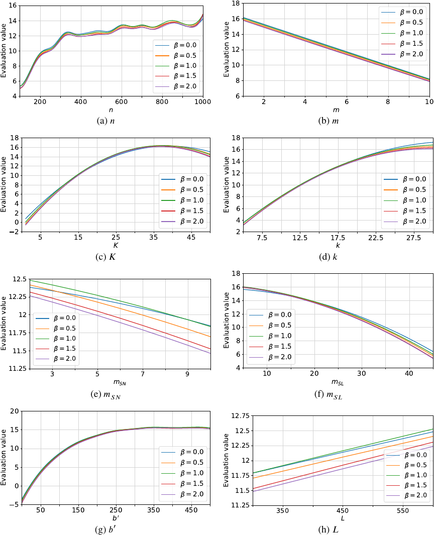
Fig. 5. Estimated evaluation values for each experimental parameter at different \(\beta\).

5.2.1. Fixed \(\alpha\) Cases

The results of the comparison are shown in Fig. 4. The vertical and horizontal axes represent evaluation values and experimental parameters, respectively. In addition, the hill-climbing method was applied to every problems that produced a feasible solution, and the estimated evaluation values based on GPR are plotted in Fig. 4.

Figure 4 shows that, overall, there is no significant difference in evaluation values among \(\alpha = 0.8\), \(\alpha = 0.85\), and \(\alpha = 0.9\). The best performance is observed for \(\alpha = 0.9\), while the worst is seen at observed for \(\alpha = 0.95\). Alternatively, if the temperature is lowered too slowly or remains high for too long, which results in a prolonged high probability of degradation, it becomes difficult to achieve a near-optimal solution. This discrepancy is especially pronounced when both the number of workers and the number of tasks are large, possibly because a larger solution space requires more time to improve the solution; if the period during which alterations are likely is extended, there will be insufficient time to reach the optimal solution. Moreover, the shorter the algorithm’s time limit, the greater the discrepancy between the results for \(\alpha = 0.95\) and those for the other \(\alpha\) values. Compared with the hill-climbing method, the proposed algorithm generally produced higher evaluation values. On average, the proposed algorithm achieved evaluation value improvements of at least 16.5%, 10.2%, 24.6%, 9.41%, 12.2%, 11.6%, and 6.84% as shown in Figs. 4(a)–(g), respectively.

5.2.2. Fixed \(\beta\) Cases

The same analysis was performed for \(\beta\), and the results are shown in Fig. 5. For comparison, we computed the evaluation values for all \(\alpha\) values with \(\beta = 0\). Note that setting \(\beta = 0\) is equivalent to applying no smoothing in the optimization. Fig. 5 indicates that the evaluation values are most favorable when \(\beta = 0\), and the difference between these values and those obtained for small \(\beta\) is trivial. Therefore, the smoothing process appears to be ineffective.

6. Conclusion

In this study, we defined a crowdsourcing team formation problem, termed the multi-team formation problem, and proposed a heuristic team formation algorithm. In addition to the skill level and budget constraints considered in previous studies, our team formation problem introduced a team size requirement. The objective function is based on density, which is a plausible measure of team compatibility derived from social networks. Furthermore, the problem assumed concurrent team formation for multiple tasks while limiting the worker load.

A simulation experiment was conducted to verify the characteristics and effectiveness of the proposed algorithm. GPR was used to elucidate the relationship between the eight experimental parameters and evaluation values. The results suggest that low values for the team size limit, degree mean, and additional budget adversely affect evaluation values. We determined that a large number of workers are necessary when both the number of tasks and the mean distribution of the required skill levels are high. The proposed algorithm has two hyperparameters: \(\alpha\), which controls the rate of temperature decrease in the simulated annealing method, and \(\beta\), which controls the smoothing degree. According to this experiment, the highest evaluation values were observed when \(\alpha = 0.9\), while variations in \(\beta\) had minimal impact. This suggests that the smoothing process implemented in the proposed algorithm is ineffective. A comparison between the proposed algorithm and the hill-climbing method demonstrates the effectiveness of the annealing method.

A limitation of this study is that we only compared the proposed algorithm with the hill-climbing method, which is a simple heuristic, as a baseline. Although this is sufficient to demonstrate the superiority of the proposed algorithm, more comprehensive comparisons with other metaheuristics, such as genetic algorithms or reinforcement learning methods, remain as future work.

There are two primary areas of future research in this field. The first is the handling of new workers in the system. In the proposed algorithm, workers who are closely connected to a social network are more likely to be selected as team members. Consequently, well-connected workers tend to be selected more often, whereas those with fewer neighboring nodes are less likely to be selected. As teamwork is implemented, the edges of the social network are updated. However, newly registered crowd workers typically have little experience with teamwork and few connections. This raises the challenge of integrating new workers into the system. One possible approach is to adjust the communication costs for edges connected to new workers, either by slightly increasing them to reflect uncertainty in their compatibility or by lowering them to give such workers additional opportunities to be selected. Alternatively, predictive models can be employed to predict and augment network connections based on worker profiles and overall social network structure. Balancing the fairness of new workers with the reliability of team performance remains an important direction for future research. The second area involves the development of a program to generate initial solutions for the proposed algorithm. Before applying an optimization algorithm based on simulated annealing, it is essential to determine whether feasible solutions satisfying all constraints exist. The current approach addresses this issue by using an external SAT solver; however, this solver requires significant computation time when the search space is large and the region of feasible solutions is small. In addition, a large solution space combined with excessive constraints can lead to file encoding errors. Therefore, we are currently developing a new algorithm to solve the constraint satisfaction problem, as described in ³⁸.

Acknowledgements

This work was supported by JSPS KAKENHI Grant Numbers JP21H03553, JP23K26329.

References

[1] K. Kashima, S. Oyama, and B. Yukino, “Human Computation and Crowdsourcing, 1st ed.,” Kodansha, 2016.
[2] G. Hertel, “Synergetic effects in working teams,” J. of Managerial Psychology, Vol.26, No.3, pp. 176-184, 2011. https://doi.org/10.1108/02683941111112622
[3] J. Hüffmeier and G. Hertel, “When the whole is more than the sum of its parts: Group motivation gains in the wild,” J. of Experimental Social Psychology, Vol.47, No.2, pp. 455-459, 2011. https://doi.org/10.1016/j.jesp.2010.12.004
[4] I. Lykourentzou, A. Antoniou, Y. Naudet, and S. P. Dow, “Personality matters: Balancing for personality types leads to better outcomes for crowd teams,” Proc. of the 19th ACM Conf. on Computer-Supported Cooperative Work & Social Computing, pp. 260-273, 2016. https://doi.org/10.1145/2818048.2819979
[5] K. L. Smart and C. Barnum, “Communication in cross-functional teams: an introduction to this special issue,” IEEE Trans. on Professional Communication, Vol.43, No.1, pp. 19-21, 2000. https://doi.org/10.1109/TPC.2000.826413
[6] A. Majumder, S. Datta, and K. V. M. Naidu, “Capacitated team formation problem on social networks,” Proc. of the 18th ACM SIGKDD Int. Conf. on Knowledge Discovery and Data Mining, pp. 1005-1013, 2012. https://doi.org/10.1145/2339530.2339690
[7] R. Kenna and B. Berche, “Managing research quality: critical mass and optimal academic research group size,” IMA J. of Management Mathematics, Vol.23, No.2, pp. 195-207, 2011. https://doi.org/10.1093/imaman/dpr021
[8] F. Khatib, F. DiMaio, F. C. Group, F. V. C. Group, S. Cooper, M. Kazmierczyk, M. Gilski, S. Krzywda, H. Zabranska, I. Pichova, J. Thompson, Z. Popović, M. Jaskolski, and D. Baker, “Crystal structure of a monomeric retroviral protease solved by protein folding game players,” Nature Structural & Molecular Biology, Vol.18, No.10, pp. 1175-1177, 2011. https://doi.org/10.1038/nsmb.2119
[9] T. Lappas, K. Liu, and E. Terzi, “Finding a team of experts in social networks,” Proc. of the 15th ACM SIGKDD Int. Conf. on Knowledge Discovery and Data Mining, pp. 467-476, 2009. https://doi.org/10.1145/1557019.1557074
[10] C.-T. Li and M.-K. Shan, “Team formation for generalized tasks in expertise social networks,” Proc. of the IEEE 2nd Int. Conf. on Social Computing, pp. 9-16, 2010. https://doi.org/10.1109/SocialCom.2010.12
[11] A. Gajewar and A. D. Sarma, “Multi-skill collaborative teams based on densest subgraphs,” Proc. of the 2012 SIAM Int. Conf. on Data Mining (SDM), pp. 165-176, 2012. https://doi.org/10.1137/1.9781611972825.15
[12] G. K. Awal and K. K. Bharadwaj, “Team formation in social networks based on collective intelligence—An evolutionary approach,” Applied Intelligence, Vol.41, No.2, pp. 627-648, 2014. https://doi.org/10.1007/s10489-014-0528-y
[13] M.-C. Juang, C.-C. Huang, and J.-L. Huang, “Efficient algorithms for team formation with a leader in social networks,” The J. of Supercomputing, Vol.66, No.2, pp. 721-737, 2013. https://doi.org/10.1007/s11227-013-0907-x
[14] K. Selvarajah, P. M. Zadeh, Z. Kobti, Y. Palanichamy, and M. Kargar, “A unified framework for effective team formation in social networks,” Expert Systems with Applications, Vol.177, Article No.114886, 2021. https://doi.org/10.1016/j.eswa.2021.114886
[15] C.-T. Li, M.-K. Shan, and S.-D. Lin, “On team formation with expertise query in collaborative social networks,” Knowledge and Information Systems, Vol.42, No.2, pp. 441-463, 2015. https://doi.org/10.1007/s10115-013-0695-x
[16] C. Dorn and S. Dustdar, “Composing near-optimal expert teams: A trade-off between skills and connectivity,” On the Move to Meaningful Internet Systems (OTM 2010), pp. 472-489, 2010. https://doi.org/10.1007/978-3-642-16934-2_35
[17] F. Farhadi, M. Sorkhi, S. Hashemi, and A. Hamzeh, “An effective expert team formation in social networks based on skill grading,” Proc. of the IEEE 11th Int. Conf. on Data Mining Workshops, pp. 366-372, 2011. https://doi.org/10.1109/ICDMW.2011.28
[18] C. Dorn, F. Skopik, D. Schall, and S. Dustdar, “Interaction mining and skill-dependent recommendations for multi-objective team composition,” Data & Knowledge Engineering, Vol.70, No.10, pp. 866-891, 2011. https://doi.org/10.1016/j.datak.2011.06.004
[19] M. Kargar, A. An, and M. Zihayat, “Efficient bi-objective team formation in social networks,” Machine Learning and Knowledge Discovery in Databases, pp. 483-498, 2012. https://doi.org/10.1007/978-3-642-33486-3_31
[20] M. Kargar, M. Zihayat, and A. An, “Finding affordable and collaborative teams from a network of experts,” Proc. of the 2013 SIAM Int. Conf. on Data Mining, pp. 587-595, 2013. https://doi.org/10.1137/1.9781611972832.65
[21] A. Anagnostopoulos, L. Becchetti, C. Castillo, A. Gionis, and S. Leonardi, “Online team formation in social networks,” Proc. of the 21st Int. Conf. on World Wide Web, pp. 839-848, 2012. https://doi.org/10.1145/2187836.2187950
[22] S. S. Rangapuram, T. Bühler, and M. Hein, “Towards realistic team formation in social networks based on densest subgraphs,” Proc. of the 22nd Int. Conf. on World Wide Web, pp. 1077-1088, 2013. https://doi.org/10.1145/2488388.2488482
[23] Y. Yang and H. Hu, “Team formation with time limit in social networks,” Proc. 2013 Int. Conf. on Mechatronic Sciences, Electric Engineering and Computer, pp. 1590-1594, 2013. https://doi.org/10.1109/MEC.2013.6885315
[24] L. Chen, Y. Ye, A. Zheng, F. Xie, Z. Zheng, and M. R. Lyu, “Incorporating geographical location for team formation in social coding sites,” World Wide Web, Vol.23, No.1, pp. 153-174, 2020. https://doi.org/10.1007/s11280-019-00712-x
[25] K. Selvarajah, A. Bhullar, Z. Kobti, and M. Kargar, “WSCAN-TFP: Weighted scan clustering algorithm for team formation problem in social network,” Proc. of the 31st Int. Florida Artificial Intelligence Research Society Conf., pp. 209-212, 2018.
[26] K. Selvarajah, P. M. Zadeh, M. Kargar, and Z. Kobti, “Identifying a team of experts in social networks using a cultural algorithm,” Procedia Computer Science, Vol.151, pp. 477-484, 2019. https://doi.org/10.1016/j.procs.2019.04.065
[27] H. Rahman, S. B. Roy, S. Thirumuruganathan, S. Amer-Yahia, and G. Das, “Task assignment optimization in collaborative crowdsourcing,” Proc. of the 2015 IEEE Int. Conf. on Data Mining, pp. 949-954, 2015. https://doi.org/10.1109/ICDM.2015.119
[28] Y. Sun, W. Tan, and Q. Zhang, “An efficient algorithm for crowdsourcing workflow tasks to social networks,” Proc. of the IEEE 20th Int. Conf. on Computer Supported Cooperative Work in Design, pp. 532-538, 2016. https://doi.org/10.1109/CSCWD.2016.7566046
[29] R. Yamamoto and K. Okamoto, “Worker organization system for collaborative crowdsourcing,” Intelligent and Transformative Production in Pandemic Times, pp. 13-22, 2023. https://doi.org/10.1007/978-3-031-18641-7_2
[30] A. Yadav, A. S. Sairam, and A. Kumar, “Concurrent team formation for multiple tasks in crowdsourcing platform,” Proc. of the 2017 IEEE Global Communications Conf., 2017. https://doi.org/10.1109/GLOCOM.2017.8255048
[31] Q. Liu, T. Luo, R. Tang, and S. Bressan, “An efficient and truthful pricing mechanism for team formation in crowdsourcing markets,” Proc. of the 2015 IEEE Int. Conf. on Communications (ICC), pp. 567-572, 2015. https://doi.org/10.1109/ICC.2015.7248382
[32] W. Wang, J. Jiang, B. An, Y. Jiang, and B. Chen, “Toward efficient team formation for crowdsourcing in noncooperative social networks,” IEEE Trans. on Cybernetics, Vol.47, No.12, pp. 4208-4222, 2017. https://doi.org/10.1109/TCYB.2016.2602498
[33] G. Barnabò, A. Fazzone, S. Leonardi, and C. Schwiegelshohn, “Algorithms for fair team formation in online labour marketplaces,” Companion Proc. of The 2019 World Wide Web Conf., pp. 484-490, 2019. https://doi.org/10.1145/3308560.3317587
[34] W. Chen, J. Yang, and Y. Yu, “Analysis on communication cost and team performance in team formation problem,” Collaborative Computing: Networking, Applications and Worksharing, pp. 435-443, 2018. https://doi.org/10.1007/978-3-030-00916-8_41
[35] M. Kargar and A. An, “Discovering top-k teams of experts with/without a leader in social networks,” Proc. of the 20th ACM Int. Conf. on Information and Knowledge Management, pp. 985-994, 2011. https://doi.org/10.1145/2063576.2063718
[36] A. Lancichinetti, S. Fortunato, and F. Radicchi, “Benchmark graphs for testing community detection algorithms,” Physical Review E, Vol.78, No.4, Article No.046110, 2008. https://doi.org/10.1103/PhysRevE.78.046110
[37] N. Tamura and M. Banbara, “Sugar: A csp to sat translator based on order encoding,” Proc. of the 2nd Int. CSP Solver Competition, pp. 65-69, 2008.
[38] R. Yamamoto and K. Okamoto, “An algorithm for solving constraint satisfaction problems in concurrent formation of expert teams,” IEICE Trans. on Information and Systems (Japanese Edition), Vol.J107-D, No.3, pp. 87-97, 2024 (in Japanese). https://doi.org/10.14923/transinfj.2023JDP7006

This article is published under a Creative Commons Attribution-NoDerivatives 4.0 Internationa License.

[B1] [1] K. Kashima, S. Oyama, and B. Yukino, “Human Computation and Crowdsourcing, 1st ed.,” Kodansha, 2016.

[B2] [2] G. Hertel, “Synergetic effects in working teams,” J. of Managerial Psychology, Vol.26, No.3, pp. 176-184, 2011. https://doi.org/10.1108/02683941111112622

[B3] [3] J. Hüffmeier and G. Hertel, “When the whole is more than the sum of its parts: Group motivation gains in the wild,” J. of Experimental Social Psychology, Vol.47, No.2, pp. 455-459, 2011. https://doi.org/10.1016/j.jesp.2010.12.004

[B4] [4] I. Lykourentzou, A. Antoniou, Y. Naudet, and S. P. Dow, “Personality matters: Balancing for personality types leads to better outcomes for crowd teams,” Proc. of the 19th ACM Conf. on Computer-Supported Cooperative Work & Social Computing, pp. 260-273, 2016. https://doi.org/10.1145/2818048.2819979

[B5] [5] K. L. Smart and C. Barnum, “Communication in cross-functional teams: an introduction to this special issue,” IEEE Trans. on Professional Communication, Vol.43, No.1, pp. 19-21, 2000. https://doi.org/10.1109/TPC.2000.826413

[B6] [6] A. Majumder, S. Datta, and K. V. M. Naidu, “Capacitated team formation problem on social networks,” Proc. of the 18th ACM SIGKDD Int. Conf. on Knowledge Discovery and Data Mining, pp. 1005-1013, 2012. https://doi.org/10.1145/2339530.2339690

[B7] [7] R. Kenna and B. Berche, “Managing research quality: critical mass and optimal academic research group size,” IMA J. of Management Mathematics, Vol.23, No.2, pp. 195-207, 2011. https://doi.org/10.1093/imaman/dpr021

[B8] [8] F. Khatib, F. DiMaio, F. C. Group, F. V. C. Group, S. Cooper, M. Kazmierczyk, M. Gilski, S. Krzywda, H. Zabranska, I. Pichova, J. Thompson, Z. Popović, M. Jaskolski, and D. Baker, “Crystal structure of a monomeric retroviral protease solved by protein folding game players,” Nature Structural & Molecular Biology, Vol.18, No.10, pp. 1175-1177, 2011. https://doi.org/10.1038/nsmb.2119

[B9] [9] T. Lappas, K. Liu, and E. Terzi, “Finding a team of experts in social networks,” Proc. of the 15th ACM SIGKDD Int. Conf. on Knowledge Discovery and Data Mining, pp. 467-476, 2009. https://doi.org/10.1145/1557019.1557074

[B10] [10] C.-T. Li and M.-K. Shan, “Team formation for generalized tasks in expertise social networks,” Proc. of the IEEE 2nd Int. Conf. on Social Computing, pp. 9-16, 2010. https://doi.org/10.1109/SocialCom.2010.12

[B11] [11] A. Gajewar and A. D. Sarma, “Multi-skill collaborative teams based on densest subgraphs,” Proc. of the 2012 SIAM Int. Conf. on Data Mining (SDM), pp. 165-176, 2012. https://doi.org/10.1137/1.9781611972825.15

[B12] [12] G. K. Awal and K. K. Bharadwaj, “Team formation in social networks based on collective intelligence—An evolutionary approach,” Applied Intelligence, Vol.41, No.2, pp. 627-648, 2014. https://doi.org/10.1007/s10489-014-0528-y

[B13] [13] M.-C. Juang, C.-C. Huang, and J.-L. Huang, “Efficient algorithms for team formation with a leader in social networks,” The J. of Supercomputing, Vol.66, No.2, pp. 721-737, 2013. https://doi.org/10.1007/s11227-013-0907-x

[B14] [14] K. Selvarajah, P. M. Zadeh, Z. Kobti, Y. Palanichamy, and M. Kargar, “A unified framework for effective team formation in social networks,” Expert Systems with Applications, Vol.177, Article No.114886, 2021. https://doi.org/10.1016/j.eswa.2021.114886

[B15] [15] C.-T. Li, M.-K. Shan, and S.-D. Lin, “On team formation with expertise query in collaborative social networks,” Knowledge and Information Systems, Vol.42, No.2, pp. 441-463, 2015. https://doi.org/10.1007/s10115-013-0695-x

[B16] [16] C. Dorn and S. Dustdar, “Composing near-optimal expert teams: A trade-off between skills and connectivity,” On the Move to Meaningful Internet Systems (OTM 2010), pp. 472-489, 2010. https://doi.org/10.1007/978-3-642-16934-2_35

[B17] [17] F. Farhadi, M. Sorkhi, S. Hashemi, and A. Hamzeh, “An effective expert team formation in social networks based on skill grading,” Proc. of the IEEE 11th Int. Conf. on Data Mining Workshops, pp. 366-372, 2011. https://doi.org/10.1109/ICDMW.2011.28

[B18] [18] C. Dorn, F. Skopik, D. Schall, and S. Dustdar, “Interaction mining and skill-dependent recommendations for multi-objective team composition,” Data & Knowledge Engineering, Vol.70, No.10, pp. 866-891, 2011. https://doi.org/10.1016/j.datak.2011.06.004

[B19] [19] M. Kargar, A. An, and M. Zihayat, “Efficient bi-objective team formation in social networks,” Machine Learning and Knowledge Discovery in Databases, pp. 483-498, 2012. https://doi.org/10.1007/978-3-642-33486-3_31

[B20] [20] M. Kargar, M. Zihayat, and A. An, “Finding affordable and collaborative teams from a network of experts,” Proc. of the 2013 SIAM Int. Conf. on Data Mining, pp. 587-595, 2013. https://doi.org/10.1137/1.9781611972832.65

[B21] [21] A. Anagnostopoulos, L. Becchetti, C. Castillo, A. Gionis, and S. Leonardi, “Online team formation in social networks,” Proc. of the 21st Int. Conf. on World Wide Web, pp. 839-848, 2012. https://doi.org/10.1145/2187836.2187950

[B22] [22] S. S. Rangapuram, T. Bühler, and M. Hein, “Towards realistic team formation in social networks based on densest subgraphs,” Proc. of the 22nd Int. Conf. on World Wide Web, pp. 1077-1088, 2013. https://doi.org/10.1145/2488388.2488482

[B23] [23] Y. Yang and H. Hu, “Team formation with time limit in social networks,” Proc. 2013 Int. Conf. on Mechatronic Sciences, Electric Engineering and Computer, pp. 1590-1594, 2013. https://doi.org/10.1109/MEC.2013.6885315

[B24] [24] L. Chen, Y. Ye, A. Zheng, F. Xie, Z. Zheng, and M. R. Lyu, “Incorporating geographical location for team formation in social coding sites,” World Wide Web, Vol.23, No.1, pp. 153-174, 2020. https://doi.org/10.1007/s11280-019-00712-x

[B25] [25] K. Selvarajah, A. Bhullar, Z. Kobti, and M. Kargar, “WSCAN-TFP: Weighted scan clustering algorithm for team formation problem in social network,” Proc. of the 31st Int. Florida Artificial Intelligence Research Society Conf., pp. 209-212, 2018.

[B26] [26] K. Selvarajah, P. M. Zadeh, M. Kargar, and Z. Kobti, “Identifying a team of experts in social networks using a cultural algorithm,” Procedia Computer Science, Vol.151, pp. 477-484, 2019. https://doi.org/10.1016/j.procs.2019.04.065

[B27] [27] H. Rahman, S. B. Roy, S. Thirumuruganathan, S. Amer-Yahia, and G. Das, “Task assignment optimization in collaborative crowdsourcing,” Proc. of the 2015 IEEE Int. Conf. on Data Mining, pp. 949-954, 2015. https://doi.org/10.1109/ICDM.2015.119

[B28] [28] Y. Sun, W. Tan, and Q. Zhang, “An efficient algorithm for crowdsourcing workflow tasks to social networks,” Proc. of the IEEE 20th Int. Conf. on Computer Supported Cooperative Work in Design, pp. 532-538, 2016. https://doi.org/10.1109/CSCWD.2016.7566046

[B29] [29] R. Yamamoto and K. Okamoto, “Worker organization system for collaborative crowdsourcing,” Intelligent and Transformative Production in Pandemic Times, pp. 13-22, 2023. https://doi.org/10.1007/978-3-031-18641-7_2

[B30] [30] A. Yadav, A. S. Sairam, and A. Kumar, “Concurrent team formation for multiple tasks in crowdsourcing platform,” Proc. of the 2017 IEEE Global Communications Conf., 2017. https://doi.org/10.1109/GLOCOM.2017.8255048

[B31] [31] Q. Liu, T. Luo, R. Tang, and S. Bressan, “An efficient and truthful pricing mechanism for team formation in crowdsourcing markets,” Proc. of the 2015 IEEE Int. Conf. on Communications (ICC), pp. 567-572, 2015. https://doi.org/10.1109/ICC.2015.7248382

[B32] [32] W. Wang, J. Jiang, B. An, Y. Jiang, and B. Chen, “Toward efficient team formation for crowdsourcing in noncooperative social networks,” IEEE Trans. on Cybernetics, Vol.47, No.12, pp. 4208-4222, 2017. https://doi.org/10.1109/TCYB.2016.2602498

[B33] [33] G. Barnabò, A. Fazzone, S. Leonardi, and C. Schwiegelshohn, “Algorithms for fair team formation in online labour marketplaces,” Companion Proc. of The 2019 World Wide Web Conf., pp. 484-490, 2019. https://doi.org/10.1145/3308560.3317587

[B34] [34] W. Chen, J. Yang, and Y. Yu, “Analysis on communication cost and team performance in team formation problem,” Collaborative Computing: Networking, Applications and Worksharing, pp. 435-443, 2018. https://doi.org/10.1007/978-3-030-00916-8_41

[B35] [35] M. Kargar and A. An, “Discovering top-k teams of experts with/without a leader in social networks,” Proc. of the 20th ACM Int. Conf. on Information and Knowledge Management, pp. 985-994, 2011. https://doi.org/10.1145/2063576.2063718

[B36] [36] A. Lancichinetti, S. Fortunato, and F. Radicchi, “Benchmark graphs for testing community detection algorithms,” Physical Review E, Vol.78, No.4, Article No.046110, 2008. https://doi.org/10.1103/PhysRevE.78.046110

[B37] [37] N. Tamura and M. Banbara, “Sugar: A csp to sat translator based on order encoding,” Proc. of the 2nd Int. CSP Solver Competition, pp. 65-69, 2008.

[B38] [38] R. Yamamoto and K. Okamoto, “An algorithm for solving constraint satisfaction problems in concurrent formation of expert teams,” IEICE Trans. on Information and Systems (Japanese Edition), Vol.J107-D, No.3, pp. 87-97, 2024 (in Japanese). https://doi.org/10.14923/transinfj.2023JDP7006