Research Paper:
Pricing Cash-or-Nothing Binary Options with Two Underlying Assets Under Default Risk
Chieh-Wen Hsu†
School of Qiaoxing Economics and Management, Fujian Polytechnic Normal University
No.1 Campus New Village, Longjiang Street, Fuqing, Fujian 350300, China
†Corresponding author

This study extended the theory of binary option pricing under default risk by extending the single underlying asset model to two underlying assets and a bilateral strike price model, while considering the correlation between different assets, focusing on the pricing analysis of cash-or-nothing binary options. The study derives a closed form options pricing formula using the Martingale method and proves that the formula is applicable to the pricing formula of binary option call and put options under default risk. Finally, numerical examples are used to analyze the characteristics and hedging value changes of binary options with two underlying assets under default risk. In addition, this study also highlights that under default risk, hedging with multiple underlying options is more difficult than general option hedging operations. This formula helps issuers to further understand the important basis for effective hedging in the issuance of multiple underlying commodities.
Binary options under default risk
1. Introduction
1.1. Study Background
Financial innovation refers to the development and implementation of innovative financial instruments, service models, trading mechanisms, and institutional norms to optimize the efficiency of market resource allocation, improve risk-sharing mechanisms, and enhance financial system functions. This study focuses on innovation in financial products. Among many financial products, binary options are a popular form of warrant. The characteristic of options is that if the underlying price falls within a predetermined price range at maturity, the holder will be paid a certain amount of money; in contrast, if the target price does not fall within this range, no amount will be paid.
In terms of the development of binary option pricing, the existing literature on model construction includes that by Thavaneswaran et al., who first introduced the fuzzy number theory framework to analyze the pricing of asset-or-nothing binary options, effectively addressing the quantification of financial market uncertainty 1. Subsequently, Qin et al. further integrated fuzzy mathematics with the long memory property of the market, assuming that the underlying asset price follows fractional Brownian motion, and derived a pricing model that is more practical and adaptable 2. Notably, Lu and Song broke through the limitations of traditional diffusion models by constructing a mixed exponential jump diffusion process and incorporating random interest rate factors to systematically explore the impact on the value of binary options 3. The latest research shows that Yang and Gao 4 established a pricing model based on the stock price dynamics model by Liu 5 that can be applied to both European and American binary options, significantly expanding the application of these derivative products. The aforementioned research has formed considerable theoretical accumulation; however, the completeness of the model for pricing issues in the context of the coexistence of multiple underlying assets and default risk can be further improved.
When financial institutions engage in options issuance, they have to bear the inherent market risks of derivative products and face the interaction of multiple operational risks such as proprietary trading, underwriting and brokerage. This risk characteristic prompts investors to evaluate the price dynamics of the underlying asset and systematically analyze the financial soundness and default risk exposure of the issuing institution during the decision-making process. Regarding the theoretical exploration of the default risk of derivative products, Johnson and Stulz innovatively identified that in over-the-counter market options, owing to the lack of clearing mechanisms, the contract value will be significantly affected by the credit risk of the issuing institution 6. Options with a possibility of default are defined as vulnerable options. The core argument is that, when the issuing institution encounters financial difficulties, the options holder becomes a residual asset claimant.
Two main theories exist for the development of default risk models: the structural and reduced-form approaches. The structural model is based on Merton’s (1974) theory of corporate value that defines it as a default event that occurs when the asset value of the issuing institution is lower than its liability. Its subsequent development includes Johnson and Stulz’s single liability assumption model that limits the liability of the issuing institution to arise only from the options contracts issued 6; Klein criticized that, in practice, issuing institutions often have multiple liability structures. Therefore, he proposed expanding their liability structure model to include the impact of other liabilities 7. Klein and Inglis further integrated interest rate risk factors and constructed a default assessment framework 8. Liu et al. extended the application of the model to binary options and explored pricing issues in a stochastic interest rate environment 9. By contrast, in the reduced model, the financial structure of a company is skipped and replaced with an intensity process to directly simulate the random occurrence characteristics of default events. This method significantly enhances the operational flexibility of the model in practical risk management.
The default triggering mechanism between structural and reduced models fundamentally differ. The structural model is based on the observability of the financial structure of a company, with the default threshold set as an endogenous variable, whereas the reduced model considers default to be an exogenous stochastic event. This method involves Jarrow and Turnbull modeling of default intensity as a Poisson process to quantify default risk premiums 10. Subsequently, Jarrow et al. introduced a credit rating migration matrix and combined it with a Markov chain to construct a dynamic default probability model for the impact on derivative pricing 11. Notably, Niu et al. broke through the limitations of linear assumptions and combined asset price dynamics with default triggering mechanisms into a jump diffusion process, using matrix Riccati differential equations to derive semi analytical solutions 12.
A theoretical disagreement exists in academia regarding the hypothesis of a correlation between the asset value of issuing institutions and the underlying asset price of options. Jarrow and Turnbull and Hull and White argued that the two were independent of each other, based on the theory that the value of warrants issued by large financial institutions was negligible relative to the overall balance sheet size, and issuing institutions typically implemented hedging strategies to eliminate the price risk of underlying assets 13,10. However, Johnson and Stulz showed that when issuing institutions did not fully hedge or had liquidity restrictions, the balance sheet contagion effect led to a significant correlation between the default risk and underlying asset risk 6. This viewpoint was supported by multiple subsequent studies, including those by Klein, Wang, and Zhou and Li, that empirically observed a positive relationship between institutional hedging costs and asset correlation 7,14,15. Shiu et al. and Wang derived vulnerable option pricing based on a basket of assets and the correlation between assets 16,17. Liu et al. further extended the model to the scenario of coexistence of stochastic interest rates and asset correlations, improving the pricing theory framework 9.
In terms of the selection of underlying assets, Qin et al., Lu and Song, and Liu et al. mainly conducted pricing research on single underlying assets and unilateral strike prices of binary options 3,9,2. Wang studied the pricing of vulnerable options with the largest or geometric mean of two underlying assets 18. Shiu et al. primarily approximated the pricing of European vulnerable options with basket warrants 16.
1.2. Research Objectives
Although theoretical developments have taken shape, the existing models still have gaps in terms of performance conditions and single underlying asset structures. This study extends binary options with default risk by Liu et al. 9 to two underlying assets and a bilateral strike price model using a structural model that considers the interdependence between the assets of issuers and the underlying assets of options. Under the bilateral strike price framework, four different strike price ranges form a three-dimensional (3D) brick. If the underlying price falls within the set brick range at maturity, the investor is paid for a certain asset. The remainder of this paper is organized as follows: Section 2 describes the evaluation model; Section 3 derives the process and composition architecture of the option pricing formula; Section 4 derives the hedging value delta from the formula; Section 5 uses numerical examples of R software to analyze the characteristics of options and hedging strategies; Section 6 finally concludes this paper.
2. Model
2.1. Model Assumptions
This study uses the model developed by Klein and Inglis as the framework, expanding from a single underlying asset and unilateral strike price to two underlying assets and a bilateral strike price model 8. The two tradable underlying stock prices (\(S\)) follow geometric Brownian motion. The dynamic process of the underlying stock prices of options can be represented as follows:
Default risk is defined as the issuer of options such as an investment bank or securities company. The bankrupt event occurs when the assets of the issuer at the expiration date (\(V_T\)) are smaller than the debts of the issuer \(D\). Once the issuer goes bankrupt, the options holder can only claim \(V_T(1-\alpha)/D\), where \(0\le \alpha \le 1\) is the cost associated with the financial distress when the issuer becomes bankrupt. Assume that the assets (\(V\)) of the warrant issuer follow a geometric Brownian motion. The dynamic process can be represented as follows:
In addition, we assume that warrants are traded under a continuous-time frame and that the markets are perfect and frictionless. The instantaneous correlations between \({W}_{{S}_1}^Q\) and \(W_V^Q\), \(W_{S_2}^Q\) and \(W_V^Q\), and \(W_{S_1}^Q\) and \(W_{S_2}^Q\) are \(\rho_{1V}\), \(\rho_{2V}\), and \(\rho_{12}\), respectively.
2.2. Type of Cash-or-Nothing Binary Options with Two Underlying Assets
2.2.1. Cash-or-Nothing Binary Options with Two Underlying Assets (Unilateral)
Cash-or-nothing binary options with two underlying assets refer to the payment of a fixed amount \(X\) to the holder at maturity if the prices of the two underlying assets fall within different unilateral exercise price ranges. The four types of cash flows at maturity \(T\) are as follows:
-
(1)
Cash-or-nothing call options with two underlying assets.
\begin{equation*} \textit{BCNC}_T= \begin{cases} X, & \mbox{if $S_{1T}>K_1$ and $S_{2T}>K_2$},\\ 0, & \mbox{otherwise},\\ \end{cases} \end{equation*} -
(2)
Cash-or-nothing put options with two underlying assets.
\begin{equation*} \textit{BCNP}_T= \begin{cases} X, & \mbox{if $S_{1T}<K_1$ and $S_{2T}<K_2$}, \\ 0, & \mbox{otherwise},\\ \end{cases} \end{equation*} -
(3)
Type I is mixed cash-or-nothing options with two underlying assets.
\begin{equation*} \textit{BCN}\left(\textrm{I}\right)_T= \begin{cases} X, & \mbox{if $S_{1T}>K_1$ and $S_{2T}<K_2$}, \\ 0, & \mbox{otherwise},\\ \end{cases} \end{equation*} -
(4)
Type II is mixed cash-or-nothing options with two underlying assets.
\begin{equation*} \textit{BCN}\left(\textrm{II}\right)_T= \begin{cases} X, & \mbox{if $S_{1T}<K_1$ and $S_{2T}>K_2$}, \\ 0, & \mbox{otherwise}.\\ \end{cases} \end{equation*}
2.2.2. Cash-or-Nothing Binary Options with Two Underlying Assets (Bilateral)
Cash-or-nothing binary options with two underlying assets refer to a fixed amount \(X\) paid to the holder at maturity if the prices of the two underlying assets fall within different strike price ranges in both directions. This can be represented as follows:
The aforementioned formula represents bilateral cash-or-nothing options with two underlying assets, whose exercise price comprises four different exercise prices, forming a 3D brick. Considering default risk, for the convenience of the deduction process, this is referred to as C-Brick options.
3. Valuation of Vulnerable Binary Options with Two Underlying Assets
3.1. Derivation of Cash-or-Nothing Options Under Default Risk
When considering the expiration date \(T\) of C-Brick options with two underlying assets, if the assets of the options issuer are less than the liabilities, the securities firm is deemed bankrupt. Once the issuing securities firm goes bankrupt, the claim rights of options investors cannot be fully recovered, and only partial compensation can be obtained after liquidation. Considering default risk, the value of European cash-or-nothing binary options with two underlying assets at maturity \(T\) can be expressed as follows:
\(X\) represents a fixed amount; \(K_1\), \(K_2\), \(K_3\), and \(K_4\) represent four different strike prices and \(K_1<K_2\), \(K_3<K_4\) form a range resembling a 3D brick; \(V_T\), \(D\) represent the assets and liabilities, respectively, of the issuing company. When \(V_T<D\), \(K_1<S_{1T}<K_2\), and \(K_3<S_{2T}<K_4\), the issuer is liquidated and the remaining value of the company is \((1-\alpha)V_T\), where \(\alpha\) is the percentage representing deadweight costs associated with financial distress and \(0\le \alpha \le 1\), where \((1-\alpha)\) is the recovery rate. The payoff for a European cash-or-nothing options with a maturity date \(T\) is \(X(1-\alpha)V_T/D\). Considering default risk and risk neutral probability measure \((\Omega,(F_t)_{0\le t\le T},Q)\), the C-Brick value can be represented as follows:
(See Appendix A for the formal derivation.)
3.2. Formulas for Cash-or-Nothing Call and Put Options
We derive the formulas for cash-or-nothing with two underlying assets call and put options from Eq. \(\eqref{eq:6}\).
Equation \(\eqref{eq:7}\) describes a call options with two underlying assets under the default risk formula.
When \(K_1\to 0\) and \(K_3\to 0\), substituting this result into Eq. \(\eqref{eq:6}\) yields
Equation \(\eqref{eq:8}\) is a put options with two underlying assets under the default risk formula.
Therefore, Eq. \(\eqref{eq:6}\) represents the general formula for pricing cash-or-nothing options with two underlying assets under default risk. When \(K_2\to \infty\), \(K_4\to \infty\), \(K_1\to 0\), and \(K_3\to 0\), Eqs. \(\eqref{eq:7}\) and \(\eqref{eq:8}\) represent the pricing formulas for call and put options with two underlying assets under default risk, respectively.
4. Delta Value of C-Brick Call Options
Equations \(\eqref{eq:9}\) and \(\eqref{eq:10}\) represent the delta value of C-Brick call options. \(\textit{Delta}_i\) is the sums of the hedging values of the \(\partial(\textit{BCNC}_1)/\partial S_i\), \(\partial(\textit{BCNC}_2)/\partial S_i\), \(\partial(\textit{BCNC}_3)/\partial S_i\), \(\partial(\textit{BCNC}_4)/\partial S_i\), with \(i=1,2\), where \(\partial(\textit{BCNC}_1)/\partial S_i\) and \(\partial(\textit{BCNC}_2)/\partial S_i\) are positive hedging values; \(\partial(\textit{BCNC}_3)/\partial S_i\) and \(\partial(\textit{BCNC}_4)/\partial S_i\) are negative hedging values, with \(i=1,2\). Similarly, \(\textit{Delta}_V\) is the sums of the hedging values of the \(\partial(\textit{BCNC}_1)/\partial V\), \(\partial(\textit{BCNC}_3)/\partial V\), \(\partial(\textit{BCNC}_4)/\partial V\).
When hedging C-Brick call options, underlying stocks \(\textit{Delta}_1\), \(\textit{Delta}_2\), and \(\textit{Delta}_V\) must be simultaneously held. Therefore, the hedging delta value may be positive or negative, and dynamic hedging is performed as the underlying price changes. Therefore, its hedging difficulty is higher than that of general option hedging operations.
5. Numerical Examples
5.1. Numerical Example Parameter Setting
The numerical example analysis used Eq. \(\eqref{eq:7}\) to analyze the characteristics of the C-Brick call options, programmed and plotted using R software. The parameter settings were based on the parameter selection by Klein 7, whereas the other parameters were selected based on the general trading conditions of the market. Generally, the issuance time of options is between six months and two years. Therefore, assuming that the expiration date of the option was one year, the risk-free interest rate was 3%, options strike price was 11–14, standard deviation of the issuer assets was 30%, and standard deviation of the two underlying assets of the options was 10%–20%. Assuming that the value of the company assets was greater than its liabilities (\(V =10\), \(D=5\), and \(V > D\)), and that no default event existed at the beginning of the option, once the issuer went bankrupt, the unit cost of asset disposal was 50%.
5.2. Numerical Example Results and Analysis
The following numerical examples were set, as presented in Table 1, with \(K_1\) \(=11\) and \(K_3\) \(=11\). The numerical analysis results were as follows.
Table 1. Definitions and values of parameters used in numerical examples.

Figure 1 shows the changes in the C-Brick call when stock prices \(S_1\) and \(S_2\) are fixed. As shown in Fig. 1, when stock price \(S_2\) was fixed, stock price \(S_1\) increased from a low to a high price, and the C-Brick call gradually increased to the highest point, because at the strike price (\(K_1=11\)), once the stock price increased to in the money, the C-Brick call value increased. Similarly, when stock price \(S_1\) was fixed, stock price \(S_2\) increased and the C-Brick call gradually increased. Certain differences existed between the two graphs, as presented in Fig. 1, mainly because the volatility of \(S_2\) (20%) was higher than that of \(S_1\) (10%); the volatility was greater than the increase in the value of security that was in line with the general nature of call options.
In Fig. 2, when stock prices \(S_1\) and \(S_2\) were fixed respectively, observe the magnitude of change in \(\textit{Delta}_1\). When stock price \(S_2\) was fixed at the strike price (\(K_1\) \(=11\)) and stock price \(S_1\) increased to in the money, \(\textit{Delta}_1\) showed a significant increase until it reached its maximum at deep in the money. Conversely, when \(S_1\) was fixed and \(S_2\) increased to deep in-the-money, \(\textit{Delta}_1\) attains its minimum value. Therefore, the changes in \(\textit{Delta}_1\) exhibit opposite trends when \(S_1\) and \(S_2\) were fixed, respectively. This was consistent with the positive correlation between \(\textit{Delta}_1\) and stock price \(S_1\) in the case of a call options.
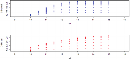
Fig. 1. Impact of \(S_1\) and \(S_2\) changes on C-Brick call.
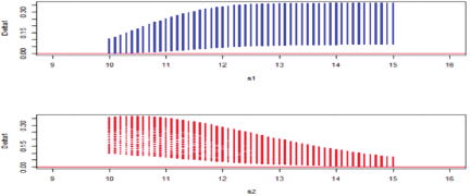
Fig. 2. Effects of price changes in \(S_1\) and \(S_2\) on \(\textit{Delta}_1\).
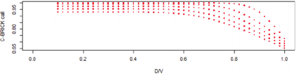
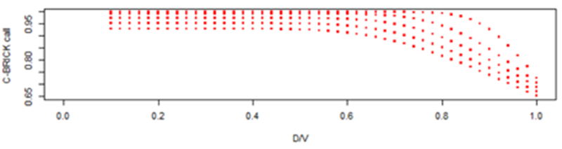
Fig. 3. Changes in the D/V on C-Brick call.
Figure 3 illustrates the variations in the debt ratio (D/V) on C-Brick calls. As shown in the figure, as the D/V gradually increased, the C-Brick call decreased from large to small. When the D/V approached one, the C-Brick call was at its minimum, indicating that the higher the company debt, the more worthless were the warrants issued.
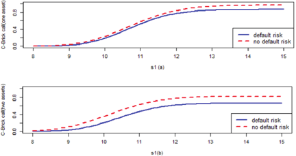
Fig. 4. Comparison of the C-Brick call between one and two underlying assets under different default risks.
Figure 4 illustrates a comparison of C-Brick call options with one and two underlying assets, considering the presence or absence of default risk. As shown in Fig. 4 (top) with \(K_1\) \(=11\) and Fig. 4 (bottom) with \(K_1\) \(=\) \(K_3\) \(=11\), with \(S_2\) \(=12\) and under unchanged other conditions, in the absence of default risk, the prices of C-Brick call options were higher, irrespective of whether one or two underlying assets existed. Moreover, irrespective of whether default risk existed, the price of C-Brick call options with a single underlying asset was higher than that with two underlying assets. This was because when default risk was considered, option purchasers were willing to buy only at a lower price. Additionally, options with two underlying assets carried greater risk than those with a single underlying asset, resulting in even lower option prices.
6. Conclusion
This study considered the pricing of dual underlying cash or free binary options under the possibility of issuer default. The general formula for dual underlying cash or free binary options under default risk was derived through a flat bet process, and the pricing formula was proved to be a call and put formula for two underlying binary options under default risk. Simultaneously, the hedging value of the option was derived from the formula that dynamically hedged with changes in the prices of the different underlying assets. Thus, option issuers could theoretically avoid option position risks through spot market operations. Finally, we used numerical examples to analyze the characteristics and hedging value changes of binary options with two targets under default risk. Additionally, under default risk, hedging with two underlying options was more difficult than general option hedging operations. However, the results of this study can be applied to provide an effective hedging basis for financial institutions when issuing binary options and to help investors reduce trading risks in their operations. Future research may consider a reduced-form approach and multiple underlying assets.
7. Appendix A.
Using Eq. \(\eqref{eq:A1}\) and changing the measure from \(Q\) to \(R\), we obtain \(S_{iT}\) and \(V_T\) as follows:
- [1] A. Thavaneswaran, S. S. Appadoo, and J. Frank, “Binary option pricing using fuzzy numbers,” J. of Applied Mathematics Letters, Vol.26, No.1, pp. 65-72, 2013. https://doi.org/10.1016/j.aml.2012.03.034
- [2] X. Qin, X. Lin, and Q. Shang, “Fuzzy pricing of binary option based on the long memory property of financial markets,” J. Intelligent and Fuzzy Systems, Vol.38, No.4, pp. 4889-4900, 2020. https://doi.org/10.3233/JIFS-191551
- [3] Y. Lu and R. Song, “Pricing of a binary option under a mixed exponential jump diffusion model,” Mathematics, Vol.12, No.20, Article No.3233, 2024. https://doi.org/10.3390/math12203233
- [4] M. Yang and Y. Gao, “Pricing formulas of binary options in uncertain financial markets,” AIMS Mathematics, Vol.8, No.10, pp. 23336-23351, 2023. https://doi.org/10.3934/math.20231186
- [5] B. Liu, “Toward uncertain finance theory,” J. of Uncertainty Analysis and Application, Vol.1, Article No.1, 2013. https://doi.org/10.1186/2195-5468-1-1
- [6] H. Johnson and R. Stulz, “The pricing of options with default risk,” J. of Finance, Vol.42, No.2, pp. 267-280, 1987. https://doi.org/10.1111/j.1540-6261.1987.tb02567.x
- [7] P. Klein, “Pricing Black-Scholes options with correlated credit risk,” J. of Banking & Finance, Vol.20, No.7, pp. 1211-1229, 1996. https://doi.org/10.1016/0378-4266(95)00052-6
- [8] P. Klein and M. Inglis, “Valuation of European options subject to financial distress and interest rate risk,” The J. of Derivatives, Vol.6, No.3, pp. 44-56, 1999. https://doi.org/10.3905/jod.1999.319118
- [9] G. X. Liu, Q. X. Zhu, and Z. W. Yan, “The Martingale approach for vulnerable binary option pricing under stochastic interest rate,” Cogent Mathematics and Statistics, Vol.4, No.1, Article No.1340073, 2017. https://doi.org/10.1080/23311835.2017.1340073
- [10] R. A. Jarrow and S. M. Turnbull, “Pricing derivatives on financial securities subject to credit risk,” J. of Finance, Vol.50, No.1, pp. 53-85, 1995. https://doi.org/10.1111/j.1540-6261.1995.tb05167.x
- [11] R. A. Jarrow, D. Lando, and S. M. Turnbull, “A Markov model for the term structures of credit risk spreads,” The Review of Financial Studies, Vol.10, No.2, pp. 481-523, 1997. https://doi.org/10.1093/rfs/10.2.481
- [12] H. Niu, Y. Xing, and Y. Zhao, “Pricing vulnerable European options with dynamic correlation between market risk and credit risk,” J. of Management Science and Engineering, Vol.5, No.2, pp. 125-145, 2020. https://doi.org/10.1016/j.jmse.2020.03.001
- [13] J. C. Hull and A. White, “The impact of default risk on the options and other derivatives securities,” J. of Banking & Finance, Vol.19, No.2, pp. 299-322, 1995. https://doi.org/10.1016/0378-4266(94)00050-D
- [14] X. Wang, “Pricing vulnerable European option with stochastic volatility correlation,” Probability in the Engineering & Informational Sciences, Vol.32, No.1, pp. 67-95, 2018. https://doi.org/10.1017/S0269964816000425
- [15] Q. Zhou and X. Li, “Vulnerable European options pricing under uncertain volatility model,” J. of Inequalities and Applications, Article No.315, pp. 1-16, 2019. https://doi.org/10.1186/s13660-019-2266-5
- [16] Y. M. Shiu, P. L. Chou, and J. W. Sheu, “A closed-form approximation for valuing European basket warrants under credit risk and interest rate risk,” Quantitative Finance, Vol.13, No.8, pp. 1211-1223, 2013. http://doi.org/10.1080/14697688.2012.741693
- [17] X. Wang, “Pricing European basket warrants with default risk under stochastic volatility models,” Applied Economics Letters, Vol.29, No.3, pp. 253-260, 2022. https://doi.org/10.1080/13504851.2020.1862745
- [18] X. Wang, “Valuing vulnerable options with two underlying assets,” Applied Economics Letters, Vol.27, No.21, pp. 1699-1760, 2020. https://doi.org/10.1080/13504851.2020.1713980
This article is published under a Creative Commons Attribution-NoDerivatives 4.0 Internationa License.