
Research Paper:
Evaluating the Circular Economy Performance of Construction and Demolition Waste Management in Taiwan: A DEA and Malmquist Index Approach
Yu-Wei Lee†
 and Yuh-Ming Lee
Institute of Natural Resource Management, National Taipei University
No.151 University Road, Sanxia District, New Taipei City 237303, Taiwan
†Corresponding author

Construction and demolition waste (CDW) is a major industrial waste stream in Taiwan. Conventional indicators such as recycling rates and treated volumes describe throughput, without directly measuring how efficiently regional systems transform resource inputs into reusable products while limiting residual waste. This study evaluates regional CDW circular-economy performance using an input-oriented data envelopment analysis (DEA) framework and the Malmquist productivity index. The original database covered 19 geographic units for 2023–2025; excluding observations with all-zero outputs, the static DEA dataset contained 53 county-year observations for 18 counties and cities. A common pooled frontier was estimated using three inputs (CDW received, licensed treatment/reuse capacity, and estimated treatment cost) and three outputs (treated/reused CDW, recycled product output, and a reciprocal transformation of residual waste). For 2023–2025, the mean Charnes-Cooper-Rhodes (CCR) efficiencies were 0.509, 0.455, and 0.461 and mean Banker-Charnes-Cooper (BCC) efficiencies 0.639, 0.598, and 0.573, respectively. Input correlations were moderate (r≤0.578). Slack analysis identified frequent treated-/reused-output shortfalls and input excesses. While the Malmquist results reveal heterogeneous regional pathways, four zero or non-finite transitions, for Kaohsiung City and Taitung County, were treated as non-interpretable numerical cases rather than as substantive productivity declines. Because the processing and output statistics include non-CDW materials and carryover inventories, scores are interpreted as relative system-level operational benchmarks. These findings support scale matching, stronger waste-to-product conversion, and region-specific management interventions. Recycled product quantity is interpreted as an operational valorization indicator rather than as a complete measure of circularity, because product quality, substitution potential, and market acceptance remain important.
Regional circular economy performance
1. Introduction
Construction and demolition waste (CDW) has become a major resource-management challenge, because construction, renovation, and demolition activities generate large material flows that contain potentially recoverable concrete, masonry, asphalt, metals, and other materials 1,2. Circular-economy approaches therefore seek both to divert CDW from disposal and return recovered materials for productive use 3,4,5,6. In Taiwan, the amount of CDW received by treatment and reuse facilities increased from approximately 2.14 million tonnes (Mt) in 2023 to 2.27 Mt in 2024 and 2.63 Mt in 2025. This increasing volume places growing pressure on treatment and reuse systems and highlights the need to improve resource recovery, recycling capacity, and circulation of secondary materials. As urban redevelopment, infrastructure renewal, and building replacement continue, effective CDW management is therefore becoming increasingly important, not only for reducing the environmental burden associated with waste treatment and disposal, but also for recovering material resources and advancing circular economy objectives in Taiwan.
Conventional indicators, such as the recycling rate, treated tonnage, and diversion rate, are informative but incomplete. They primarily describe material throughput without revealing whether a regional system relies on excessive infrastructure or cost inputs or whether the treated material is converted into usable secondary products. A high recovered tonnage does not necessarily imply high circularity, if the material quality, retained value, substitution of virgin materials, or downstream market acceptance are weak 4,5,6. Accordingly, this study treats recycled product output as an operational indicator of waste-to-product valorization, rather than as a complete circularity metric.
Data envelopment analysis (DEA) is well suited to multi-input, multi-output environmental systems because it benchmarks relative efficiency without imposing a predetermined production function 7,8. It has recently been applied to evaluate the territorial efficiency of circular economy systems 9. In waste-management applications, it has been used to evaluate cost, technical, environmental, and scale efficiency 10,11,12,13. Dynamic productivity can be evaluated using the Malmquist index, which decomposes productivity change into efficiency change (\(\mathit{EC}\)) and technological change (\(\mathit{TC}\)) 14.
Against this background, this study integrates Charnes-Cooper-Rhodes (CCR) and Banker-Charnes-Cooper (BCC) DEA, slack analysis, and Malmquist decomposition to evaluate regional CDW management in Taiwan. The findings contribute to (1) benchmarking subnational CDW systems on a common multiyear frontier, (2) incorporating recycled product output together with residual waste to move beyond throughput-only indicators, and (3) distinguishing static inefficiency from dynamic changes in efficiency and technology. The objective of the study was benchmarking and structural diagnosis, rather than causal estimation.
2. Literature Review
2.1. CDW Management and Circular Economy
CDW circular-economy research consistently emphasizes recovery, reuse, recycling, secondary-material production, and market uptake 1,3,4,5,6. López Ruiz et al. 5 organize circular strategies across the construction life cycle and identify recirculation of recovered materials as a key pathway. Purchase et al. 4 highlight technical, regulatory, economic, social, and market barriers, whereas Papamichael et al. 3 emphasize that CDW management must be evaluated across the broader material cycle. These studies support product-oriented indicators but also caution against equating recovered quantity with circularity when quality and market functionality are not represented.
2.2. DEA in Environmental and Waste Management
While the CCR model estimates overall technical efficiency under constant returns to scale, the BCC model permits variable returns to scale and isolates pure technical efficiency 7,8, and their ratio reveals scale efficiency. DEA has been applied to municipal waste services and environmental systems to compare performance across jurisdictions and identify cost, operational, and scale inefficiencies 10,11,12,13. Because DEA constructs a frontier from observed data, the results are sensitive to variable selection, dimensionality, data quality, and atypical observations; therefore, transparent specifications and diagnostic reporting are important 15.
2.3. Dynamic Productivity and Research Gap
The Malmquist productivity index extends frontier analysis across time by decomposing productivity change into efficiency and technological changes 14. Recent studies of waste-management applications have revealed that recycling and sustainable-waste productivity can evolve through different combinations of catch-up and frontier movements 16,17. Nevertheless, most waste DEA studies have focused on municipal solid waste or aggregate environmental performance rather than on subnational CDW systems. The present study therefore combines static DEA, slack diagnostics, and Malmquist decomposition, while explicitly incorporating recycled product output and residual waste.
3. Methodology
3.1. Study Units, Analytical Sample, and Pooled Frontier
The original database covered 19 Taiwanese counties and cities for the period 2023–2025. Preprocessing excluded county-year observations for which treated/reused CDW, recycled product output, and residual waste were simultaneously zero. Chiayi City had all-zero outputs in the available years and was therefore not included in the final DEA dataset, and for 2023, Hsinchu County was excluded under the same criterion. The final static DEA dataset comprised 53 county-year observations from 18 geographic units (17 for 2023 and 18 for both 2024 and 2025). Each county-year observation period was evaluated against the common pooled frontier.
With \({m=3}\) inputs and \({s=3}\) outputs, the commonly used DEA dimensionality heuristic \(n \geq \max\{{m*s}, {3(m+s)}\}\) proposed by Cooper et al. 18 gives a minimum of 18 observations 15. The pooled DEA contains 53 county-year observations and therefore exceeds this heuristic, although the observations represent only 18 geographic systems over a short time period.
3.2. Variables, Construction, and Official Data Sources
Data for 2023–2025 were compiled from the official information systems maintained by the Resource Circulation Administration, Ministry of Environment, Taiwan. CDW received, treated/reused CDW, recycled product output, and residual waste were obtained from statistical data in the Industrial Waste Report and Management Information System 19. The licensed treatment/reuse capacity was compiled from the Waste Clearance and Disposal Organization Service Management Information System and the Resource Recycling Management Information System. The treatment-cost input was estimated as the relevant treatment/output quantity multiplied by the corresponding unit treatment fee obtained from the Waste Clearance and Disposal Organization Service Management Information System. The resulting annual cost was calculated in New Taiwan dollars per year (NT$/year). Before DEA estimation, this variable was divided by \(10^{6}\); the values supplied to DEA are therefore numerically expressed in million NT$/year (this unit rescaling does not change the economic definition of the variable). Accordingly, this variable represents an estimated treatment-cost input rather than an audited financial expenditure by individual local governments or facilities. “CDW received” denotes CDW received during the reporting year, whereas “treated/reused CDW” denotes the total material entering treatment or reuse processes, including non-CDW materials and inventories carried over from previous periods. “Recycled product output” and “residual waste” are the corresponding quantities generated by these processes. Treated/reused CDW is approximately equal to recycled product output plus residual waste. These related indicators describe processing throughput, product recovery, and residual generation rather than independent material quantities (Table 1).
| Role | Variable | Definition | Unit | Source |
| Input | CDW received | Annual quantity of CDW received during the reporting year | t/year | (1) |
| Input | Licensed capacity | Total licensed treatment/reuse capacity | t/year | (2), (3) |
| Input | Estimated treatment cost | Treatment/output quantity \(\times\) unit treatment fee |
NT$/year in source data; divided by \(10^6\) before DEA |
(2) |
| Desirable output | Treated/reused CDW | Annual quantity of all materials entering treatment/reuse, including non-CDW materials and prior-period inventories | t/year | (1) |
| Desirable output | Recycled product output | Annual quantity of recycled products generated from treated/reused materials, including non-CDW materials and prior-period inventories | t/year | (1) |
| Undesirable output (transformed for DEA) | Residual waste | Annual residual quantity from treatment/reuse of all materials, including non-CDW materials and prior-period inventories; entered as \(1/(\textrm{residual waste}+1)\) | t/year before transformation | (1) |
3.3. DEA Model Specification
An input-oriented DEA model was adopted because the analytical question was whether the observed outputs could be achieved with lower resource inputs. The CCR model assumes constant returns to scale and estimates overall technical efficiency, whereas the BCC model adds a convexity constraint and estimates pure technical efficiency under variable returns to scale 7,8.
For the evaluated decision-making unit \(o\), let \(\theta\) denote the input-oriented efficiency score. The input-oriented CCR envelopment model is given as follows:
The BCC model adds \({\sum_{j} \lambda_{j} =1}\). Scale efficiency is calculated as \({\mathit{SE} = {\theta_{\mathit{CCR}}}/{\theta_{\mathit{BCC}}}}\). In the implemented input-oriented CCR/BCC models, \({0<\theta \leq 1}\) and \({\theta = 1}\) denotes frontier efficiency. Super-efficiency was calculated only as an auxiliary frontier diagnostic and was not substituted for the reported CCR/BCC scores.
3.4. Undesirable Output Transformation, Zero Treatment, and Extreme Observations
Residual waste was defined as an undesirable output. Because the implemented standard DEA output matrix treats larger output values as preferable, residual waste was converted to a desirable-form indicator using the reciprocal transformation \({b^{*} = {1/(b+c)}}\), where \(b\) denotes residual waste and \({c=1}\). Therefore, a lower residual quantity produces a higher transformation value. Consequently, the DEA model operates on the transformed indicator rather than directly on the raw residual waste. Non-positive CDW received and estimated-cost values were replaced by 0.0001, capacity values below 1 were set to 1, and the cost variable was divided by \(10^{6}\). No observation was removed solely because it was a statistical outlier. Super-efficiency diagnostics were used to identify influential frontier observations; infinite super-efficiency solutions were flagged and set to missing only for summary reporting, without altering the underlying CCR/BCC results.
3.5. Input-Correlation Diagnostic
To address possible redundancy among the inputs, Pearson’s correlations were calculated using the 53 final county-year observations. Correlation analysis was used as a redundancy diagnostic, rather than as a regression-style multicollinearity test.
3.6. Malmquist Productivity Index
The Malmquist productivity index was estimated using the same input/output structure. \({\mathit{MI}>1}\) indicates a productivity improvement and \({\mathit{MI}<1}\) a productivity decline; \(\mathit{EC}\) reflects movement toward or away from the frontier; and \(\mathit{TC}\) represents a shift in the frontier 14. \(\mathit{MI}\) was interpreted based on \(\mathit{EC}\) and \(\mathit{TC}\). A diagnostic review identified four zero or non-finite transitions (for Kaohsiung City in 2024 and 2025 and Taitung County in 2024 and 2025). The estimation procedure removed baseline rows with missing \(\mathit{MI}\) values and converted infinite \(\mathit{MI}\)/\(\mathit{EC}\)/\(\mathit{TC}\) values into missing values. However, it did not automatically remove finite zero-valued \(\mathit{MI}\) or \(\mathit{TC}\) estimates. These transitions are reported separately and are not interpreted as literal zero productivity changes. Consequently, Hsinchu County had one interpretable transition in the diagnostic summary, whereas most other regions had two transitions.
3.7. Software and Analytical Scope
All the DEA, slack, super-efficiency, and Malmquist calculations were implemented in R using the Benchmarking package. Slack analysis was performed with respect to the BCC solution using slack(x, y, e=dea_bcc); thus, the reported slacks were BCC-based input excesses and output shortfalls after radial adjustment. The analysis used dea(..., RTS="crs", ORIENTATION="in") for CCR, dea(..., RTS="vrs", ORIENTATION="in") for BCC, sdea(...) for super-efficiency, slack(...) for slack diagnostics, and malmquist(...) for productivity analysis. No second-stage regression was performed, because the objective was benchmarking rather than causal estimation and because conventional inference using estimated DEA scores requires strong assumptions and specialized procedures 20,21,22.
4. Results
4.1. Descriptive Statistics and Input Correlation
The input-correlation diagnostic yielded \({r=0.572}\) for CDW received versus licensed capacity, \({r=0.578}\) for CDW received versus estimated treatment costs, and \({r=0.275}\) for licensed capacity versus estimated treatment costs. This indicates that the relationship between the received volume and licensed capacity was moderate rather than near-perfect. Because these three inputs represent conceptually distinct dimensions—realized processing burden, authorized infrastructure, and estimated treatment cost—all three were retained (Table 2).
| Variable | Mean | SD | Min | Median | Max |
| CDW received | 130532.89 | 154859.76 | 2926.96 | 35451.22 | 561255.53 |
| Licensed capacity | 799153.90 | 922365.61 | 28386.00 | 304800.00 | 3203970.00 |
| Estimated treatment cost | 2006.02 | 4175.93 | 15.06 | 515.73 | 18550.11 |
| Treated/reused CDW | 438183.68 | 568241.26 | 7228.18 | 253073.50 | 2784866.10 |
| Recycled product output | 405024.06 | 571265.15 | 3634.01 | 229118.89 | 2902384.41 |
| Residual waste | 15992.24 | 25135.82 | 142.47 | 5439.44 | 124575.48 |
Units: t/year, except estimated treatment cost [million NT$/year]; residual waste is shown before transformation.
| Year | N |
CCR mean |
CCR SD |
BCC mean |
BCC SD |
\(\mathit{SE}\) mean |
| 2023 | 17 | 0.509 | 0.285 | 0.639 | 0.307 | 0.826 |
| 2024 | 18 | 0.455 | 0.287 | 0.598 | 0.321 | 0.794 |
| 2025 | 18 | 0.461 | 0.263 | 0.573 | 0.267 | 0.833 |
Note: \(\mathit{SE}\), scale efficiency.
4.2. Static DEA Performance Under CCR and BCC
For 2023, 2024, and 2025, the mean CCR efficiencies were 0.509, 0.455, and 0.461 and the mean BCC efficiencies were 0.639, 0.598, and 0.573, respectively. Mean scale efficiency ranged from 0.794 to 0.833 (Table 3). The persistent gap between the CCR and BCC scores indicates that scale-related effects contributed materially to overall inefficiency.
Taitung County has a mean BCC score of 1.000, followed by Keelung City (0.999), Yunlin County (0.918), Kaohsiung City (0.855), Changhua County (0.851), and Pingtung County (0.820). The lowest mean BCC scores were observed in Taipei City (0.158), New Taipei City (0.161), and Taichung City (0.270). These scores are relative to the pooled frontier and should not be interpreted as absolute measures of environmental quality (Table 4 and Fig. 1).
| Rank | Region | CCR | BCC | \(\mathit{SE}\) | Years |
| 1 | Taitung County | 0.838 | 1.000 | 0.838 | 3 |
| 2 | Keelung City | 0.239 | 0.999 | 0.239 | 3 |
| 3 | Yunlin County | 0.902 | 0.918 | 0.981 | 3 |
| 4 | Kaohsiung City | 0.579 | 0.855 | 0.683 | 3 |
| 5 | Changhua County | 0.834 | 0.851 | 0.976 | 3 |
| 6 | Pingtung County | 0.815 | 0.820 | 0.992 | 3 |
| 7 | Miaoli County | 0.730 | 0.753 | 0.970 | 3 |
| 8 | Chiayi County | 0.479 | 0.724 | 0.653 | 3 |
| 9 | Hualien County | 0.215 | 0.638 | 0.336 | 3 |
| 10 | Yilan County | 0.469 | 0.563 | 0.828 | 3 |
| 11 | Nantou County | 0.444 | 0.531 | 0.818 | 3 |
| 12 | Tainan City | 0.479 | 0.482 | 0.993 | 3 |
| 13 | Hsinchu County | 0.309 | 0.385 | 0.771 | 2 |
| 14 | Taoyuan City | 0.282 | 0.356 | 0.788 | 3 |
| 15 | Hsinchu City | 0.294 | 0.312 | 0.943 | 3 |
| 16 | Taichung City | 0.263 | 0.270 | 0.975 | 3 |
| 17 | New Taipei City | 0.152 | 0.161 | 0.942 | 3 |
| 18 | Taipei City | 0.154 | 0.158 | 0.974 | 3 |
Note: \(\mathit{SE}\), scale efficiency.
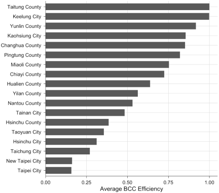
Fig. 1. Regional ranking by mean BCC efficiency.
4.3. Slack Analysis
Positive treated-/reused-output slack occurred in 79.2% of the observations. On the input side, CDW-received slack occurred in 62.3%, estimated treatment-cost slack in 45.3%, and licensed-capacity slack in 35.8% of the observations. Recycled-product-output slack was less frequent (9.4%) but was substantial for the selected observations (Table 5). Because the slack magnitudes are expressed in different native or transformed units, the raw magnitudes should not be compared directly across variables.
| Slack | Mean | SD | Median | Max | Positive [%] |
| CDW received | 20251.654 | 38893.670 | 3870.220 | 210092.934 | 62.3 |
| Licensed capacity | 90980.121 | 187989.979 | 0.000 | 728336.397 | 35.8 |
| Estimated treatment cost | 257.662 | 608.485 | 0.000 | 3061.989 | 45.3 |
| Treated/reused CDW | 53561.634 | 66786.792 | 27978.325 | 253142.016 | 79.2 |
| Recycled product output | 2874.122 | 11410.865 | 0.000 | 63051.281 | 9.4 |
| Transformed residual output | 0.001 | 0.001 | 0.000 | 0.005 | 79.2 |
4.4. Dynamic Productivity Change
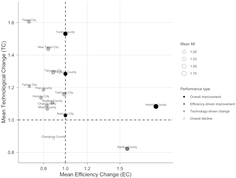
Across valid transitions, the mean \(\mathit{MI}\) was 1.060 for 2024 and 1.090 for 2025 (Table 6). For 2024, mean \(\mathit{TC}\) (1.350) exceeded mean \(\mathit{EC}\) (0.805), whereas for 2025, both mean \(\mathit{EC}\) (1.064) and \(\mathit{TC}\) (1.032) exceeded 1 (Fig. 2). Hsinchu County had the largest valid county mean \(\mathit{MI}\) (1.983), with \({\mathit{EC}=1.831}\) and \({\mathit{TC}=1.083}\). However, this estimate is based on only one valid transition and should therefore be interpreted as a single-period change rather than as a stable three-year trend. Changhua County had \({\mathit{MI}=0.790}\), \({\mathit{EC}=0.891}\), and \({\mathit{TC}=0.886}\) across the two valid transitions, indicating a decline in both components relative to the frontier (Table 7).
Four transitions were not interpreted because their \(\mathit{MI}\) and \(\mathit{TC}\) scores were zero or non-finite: Kaohsiung City (2024, 2025) and Taitung County (2024, 2025). They are reported as numerical/undefined cases rather than as genuine zero productivity changes.
| Year | N valid | \(\mathit{MI}\) mean | \(\mathit{EC}\) mean | \(\mathit{TC}\) mean |
| 2024 | 15 | 1.060 | 0.805 | 1.350 |
| 2025 | 16 | 1.090 | 1.064 | 1.032 |
Note: \(\mathit{EC}\), efficiency change; \(\mathit{TC}\), technological change.
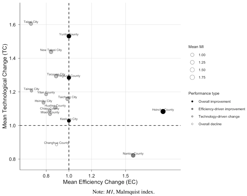
Fig. 2. Mean efficiency change (\(\mathit{EC}\)) versus mean technological change (\(\mathit{TC}\)) for interpretable regional transitions.
| Rank | Region | Valid transitions | \(\mathit{MI}\) | \(\mathit{EC}\) | \(\mathit{TC}\) |
| 1 | Hsinchu County | 1 | 1.983 | 1.831 | 1.083 |
| 2 | Yunlin County | 2 | 1.531 | 1.000 | 1.531 |
| 3 | Nantou County | 2 | 1.313 | 1.567 | 0.822 |
| 4 | Pingtung County | 2 | 1.284 | 1.000 | 1.284 |
| 5 | New Taipei City | 2 | 1.141 | 0.842 | 1.438 |
| 6 | Taichung City | 2 | 1.135 | 0.988 | 1.158 |
| 7 | Taoyuan City | 2 | 1.115 | 0.887 | 1.294 |
| 8 | Keelung City | 2 | 1.028 | 1.000 | 1.028 |
| 9 | Taipei City | 2 | 0.997 | 0.665 | 1.605 |
| 10 | Hualien County | 2 | 0.972 | 0.879 | 1.107 |
| 11 | Yilan County | 2 | 0.900 | 0.799 | 1.186 |
| 12 | Chiayi County | 2 | 0.898 | 0.830 | 1.090 |
| 13 | Miaoli County | 2 | 0.898 | 0.833 | 1.068 |
| 14 | Hsinchu City | 2 | 0.870 | 0.776 | 1.135 |
| 15 | Tainan City | 2 | 0.805 | 0.670 | 1.206 |
| 16 | Changhua County | 2 | 0.790 | 0.891 | 0.886 |
Note: \(\mathit{EC}\), efficiency change; \(\mathit{TC}\), mean technological change.
5. Discussion
Based on these findings, CDW circular-economy performance cannot be inferred from throughput or recycling rates alone. The fact that the BCC scores were systematically higher than the CCR scores indicates that scale mismatch is an important component of the observed inefficiency. This is consistent with the conceptual distinction between overall technical efficiency and pure technical efficiency in CCR/BCC DEA 7,8, and with the findings of municipal-waste studies showing that operational scale can materially affect eco-efficiency 11. The implication is not that every region should reduce its capacity; rather, capacity should be assessed against actual material flows and output conversion.
Potential redundancy among the input variables was quantitatively examined. The correlations between CDW received and licensed capacity, between CDW received and estimated treatment costs, and between licensed capacity and estimated treatment costs were 0.572, 0.578, and 0.275, respectively. These associations were meaningful but moderate, rather than near-perfect. Retaining all three of these inputs preserves their distinct concepts: the actual processing burden, the authorized infrastructure, and the estimated treatment cost. Nevertheless, because DEA discrimination can weaken as dimensionality increases, the limited geographic sample remains an explicit limitation 15.
The inclusion of recycled product output shifts attention from the treatment alone toward material valorization. However, recycled product output measures quantity, not product quality or market functionality. Circular economy research emphasizes the importance of retained value, quality, substitution potential, and functioning secondary-material markets 3,4,5,6. Accordingly, this study does not claim that a larger recycled-product tonnage is automatically more circular; rather, it uses product output as an observable operational proxy for waste-to-product conversion, within the available official dataset. The processing-throughput and recycled product indicators are therefore interpreted as related stages of material recovery, rather than as independent material flows.
The Malmquist decomposition findings provide a dynamic perspective consistent with that of prior research on waste productivity. Llanquileo-Melgarejo and Molinos-Senante 16 found that productivity and eco-productivity can be driven by different combinations of efficiency and technical change. Halkos and Aslanidis 17 used Malmquist decomposition to distinguish between efficiency and technological components in sustainable waste management. Here, the valid transitions for 2024 were predominantly associated with technological change, whereas for 2025, both the mean \(\mathit{EC}\) and mean \(\mathit{TC}\) were \({>}1\). This suggests that system-wide frontier movement does not automatically produce equivalent catch-up by every regional system.
The findings for Hsinchu County illustrate why regional interpretation should be tied to the observed input–output changes rather than to unsupported causal claims. Between the valid 2024 and 2025 observations for this county, treated/reused CDW increased from approximately 105,246 to 274,195 t and recycled product output from approximately 102,961 to 269,963 t, while licensed capacity remained at 234,540 t/year. The resulting strong \(\mathit{EC}\) component is therefore consistent with the improved input–output alignment relative to the frontier. As only one valid Malmquist transition was available for Hsinchu County, this change reflects a marked single-period improvement rather than a persistent trend.
Changhua County exhibited a different pattern: Its mean \(\mathit{MI}\) was 0.790, with \({\mathit{EC}=0.891}\) and \({\mathit{TC}=0.886}\) across the two valid transitions. BCC efficiency declined from 1.000 for 2023 to 0.637 for 2025, while received volume and estimated treatment cost both increased. This pattern is consistent with a weaker relative input–output alignment and a less favorable frontier position. However, this should not be interpreted as reflecting deficiency in local governance, because DEA is a benchmarking method and the model does not identify causal determinants.
Compared with the findings of previous DEA studies on waste, these findings reinforce three broader observations: First, waste-management and circular-economy efficiency is heterogeneous across jurisdictions 9,10,11,12; second, scale effects can be substantial and should therefore be separated from pure technical efficiency 11; and third, productivity change can be driven by technology, efficiency catch-up, or both 16,17. The municipal-solid-waste situation of Taiwan differs from that of many other locations because its production structure currently focuses specifically on CDW treatment or reuse and includes recycled product output and residual waste. These institutional and material-flow differences limit direct comparison of numerical efficiency scores across studies.
6. Limitations and Future Work
Several limitations should be noted. First, although the pooled DEA dataset contains 53 county-year observations and exceeds a common dimensionality heuristic for three inputs and three outputs, the observations represent repeated measurements for only 18 geographic systems over a short period; this may limit the discriminatory power of the pooled frontier; consequently, the frontier status and rankings should be interpreted cautiously. Second, DEA is sensitive to atypical observations; however, statistical outliers were not excluded here. Third, the reciprocal residual-waste transformation with \({c=1}\) is a pragmatic implementation within a standard DEA framework. No formal sensitivity analysis of alternative DEA specifications was conducted; alternative undesirable-output treatments or input/output selections may therefore produce somewhat different frontiers and efficiency estimates. Fourth, the statistical coverage of CDW received differs from that of the processing and output indicators, which include non-CDW materials and carryover inventories, and the approximately balanced processing and output quantities are interdependent; the efficiency estimates thus reflect relative system-level operational performance rather than CDW-specific material conversion efficiency. Fifth, the estimated treatment cost is constructed from the treatment/output quantity and unit treatment fees rather than from audited facility-level expenditure. Sixth, recycled product quantity does not directly measure product quality, price, certification, virgin-material substitution, or market absorption. Seventh, transportation variables were not included, because complete and comparable regional transport-flow data were unavailable. Eighth, the short time-frame of the data limits long-run Malmquist interpretation, and four zero/non-finite transitions were treated as numerical/undefined cases rather than as substantive productivity values.
Future research should extend the time series, incorporate product-quality and market-absorption indicators, test alternative undesirable-output DEA formulations, and evaluate robustness under alternative input/output sets. With a longer and more stable dataset, bootstrap-based inference or carefully specified second-stage methods may also be considered 20,21,22.
7. Conclusion
Based on these findings, the regional CDW performance of Taiwan is heterogeneous and cannot be adequately represented using treated tonnage or recycling rates alone. The combined CCR/BCC, slack, and Malmquist framework applied here identified scale mismatches, output shortfalls, and different dynamic pathways across regions. The diagnostics reveal that the three inputs are not near-duplicates and clarify that the implemented static DEA evaluates 53 county-year observations on a common pooled frontier. While recycled product output is useful as an operational valorization indicator, it should be interpreted together with quality and market considerations.
The policy implication of these findings is not simply to expand treatment capacity, but to improve scale matching, waste-to-product conversion, and region-specific operational alignment. These reported efficiency and productivity measures are therefore interpreted as relative operational benchmarks for CDW management-related treatment and reuse systems and not as CDW-specific material conversion rates.
Footnotes
(1) https://waste.moenv.gov.tw/RWD/Statistics/?page=Year1 [Accessed April 21, 2026]
(2) https://waste1.moenv.gov.tw/Grant/GS-UC60/QryGrantData.aspx [Accessed April 21, 2026]
(3) https://rms.moenv.gov.tw/RMS/ [Accessed April 21, 2026]
- [1] N. Elshaboury, A. Al-Sakkaf, E. M. Abdelkader, and G. Alfalah, “Construction and demolition waste management research: A science mapping analysis,” Int. J. Environ. Res. Public Health, Vol.19, No.8, Article No.4496, 2022. https://doi.org/10.3390/ijerph19084496
- [2] European Commission, Directorate-General for Internal Market, Industry, Entrepreneurship and SMEs, A. Oberender et al., “EU construction & demolition waste management protocol including guidelines for pre-demolition and pre-renovation audits of construction works—Updated edition 2024,” Publications Office of the European Union, 2024. https://doi.org/10.2873/77980
- [3] I. Papamichael, I. Voukkali, P. Loizia, and A. A. Zorpas, “Construction and demolition waste framework of circular economy: A mini review,” Waste Manag. Res., Vol.41, No.12, pp. 1728-1740, 2023. https://doi.org/10.1177/0734242X231190804
- [4] C. K. Purchase et al., “Circular economy of construction and demolition waste: A literature review on lessons, challenges, and benefits,” Materials, Vol.15, No.1, Article No.76, 2022. https://doi.org/10.3390/ma15010076
- [5] L. A. López Ruiz, X. Roca Ramón, and S. Gassó Domingo, “The circular economy in the construction and demolition waste sector – A review and an integrative model approach,” J. Clean. Prod., Vol.248, Article No.119238, 2020. https://doi.org/10.1016/j.jclepro.2019.119238
- [6] E. Iacovidou, J. N. Hahladakis, and P. Purnell, “A systems thinking approach to understanding the challenges of achieving the circular economy,” Environ. Sci. Pollut. Res., Vol.28, No.19, pp. 24785-24806, 2021. https://doi.org/10.1007/s11356-020-11725-9
- [7] A. Charnes, W. W. Cooper, and E. Rhodes, “Measuring the efficiency of decision making units,” Eur. J. Oper. Res., Vol.2, No.6, pp. 429-444, 1978. https://doi.org/10.1016/0377-2217(78)90138-8
- [8] R. D. Banker, A. Charnes, and W. W. Cooper, “Some models for estimating technical and scale inefficiencies in data envelopment analysis,” Manag. Sci., Vol.30, No.9, pp. 1078-1092, 1984. https://doi.org/10.1287/mnsc.30.9.1078
- [9] I. Marjanović, J. J. Stanković, J. Östh, M. Marković, and M. Stanojević, “Insight into territorial efficiency of circular economy through data envelopment analysis,” Front. Environ. Sci., Vol.13, Article No.1494184, 2025. https://doi.org/10.3389/fenvs.2025.1494184
- [10] N. Rogge and S. De Jaeger, “Measuring and explaining the cost efficiency of municipal solid waste collection and processing services,” Omega, Vol.41, No.4, pp. 653-664, 2013. https://doi.org/10.1016/j.omega.2012.09.006
- [11] P. Llanquileo-Melgarejo and M. Molinos-Senante, “Evaluation of economies of scale in eco-efficiency of municipal waste management: An empirical approach for Chile,” Environ. Sci. Pollut. Res., Vol.28, No.22, pp. 28337-28348, 2021. https://doi.org/10.1007/s11356-021-12529-1
- [12] G. Halkos and K. N. Petrou, “Assessing 28 EU member states’ environmental efficiency in national waste generation with DEA,” J. Clean. Prod., Vol.208, pp. 509-521, 2019. https://doi.org/10.1016/j.jclepro.2018.10.145
- [13] C.-W. Huang, Y.-H. Chiu, W.-T. Fang, and N. Shen, “Assessing the performance of Taiwan’s environmental protection system with a non-radial network DEA approach,” Energy Policy, Vol.74, pp. 547-556, 2014. https://doi.org/10.1016/j.enpol.2014.06.023
- [14] R. Färe, S. Grosskopf, M. Norris, and Z. Zhang, “Productivity growth, technical progress, and efficiency change in industrialized countries,” Am. Econ. Rev., Vol.84, No.1, pp. 66-83, 1994.
- [15] R. G. Dyson et al., “Pitfalls and protocols in DEA,” Eur. J. Oper. Res., Vol.132, No.2, pp. 245-259, 2001. https://doi.org/10.1016/S0377-2217(00)00149-1
- [16] P. Llanquileo-Melgarejo and M. Molinos-Senante, “The impact of recycling on the productivity of Municipal Solid Waste: A comparison of the Malmquist and Malmquist-Luenberger Productivity Indexes,” Int. J. Sustain. Eng., Vol.16, No.1, pp. 236-247, 2023. https://doi.org/10.1080/19397038.2023.2256382
- [17] G. E. Halkos and P.-S. C. Aslanidis, “Monitoring sustainable waste management in OECD countries: A Malmquist productivity approach,” Waste Manag., Vol.190, pp. 623-631, 2024. https://doi.org/10.1016/j.wasman.2024.10.035
- [18] W. W. Cooper, L. M. Seiford, and K. Tone, “Data Envelopment Analysis: A Comprehensive Text with Models, Applications, References and DEA-Solver Software,” 2nd edition, Springer, 2007. https://doi.org/10.1007/978-0-387-45283-8
- [19] Ministry of Environment, Taiwan, “Industrial waste report and management information system—Annual statistics,” 2026. https://waste.moenv.gov.tw/RWD/Statistics/?page=Year1 [Accessed April 21, 2026]
- [20] L. Simar and P. W. Wilson, “Estimation and inference in two-stage, semi-parametric models of production processes,” J. Econom., Vol.136, No.1, pp. 31-64, 2007. https://doi.org/10.1016/j.jeconom.2005.07.009
- [21] L. Simar and P. W. Wilson, “Two-stage DEA: Caveat emptor,” J. Prod. Anal., Vol.36, No.2, pp. 205-218, 2011. https://doi.org/10.1007/s11123-011-0230-6
- [22] R. D. Banker and R. Natarajan, “Evaluating contextual variables affecting productivity using data envelopment analysis,” Oper. Res., Vol.56, No.1, pp. 48-58, 2008. https://doi.org/10.1287/opre.1070.0460
This article is published under a Creative Commons Attribution-NoDerivatives 4.0 Internationa License.