
Research Paper:
Gated Hybrid Network Using CRNN and RNN Models for Time-Series Forecasting and Case Studies
Takayuki Kataoka*1,†
 , Tomonari Yomono*2, Sho Yamamoto*3
, and Takashi Nishi*4
*1Kindai University
1 Takaya Umenobe, Higashihiroshima, Hiroshima 739-2116, Japan
†Corresponding author
*2Dai Nippon Printing Co., Ltd.
Tokyo, Japan
*3Kindai University
Higashiosaka, Japan
*4Mazda Motor Corporation
Fuchu-cho, Japan

Time-series forecasting is a critical challenge in industrial applications such as inventory management and energy planning. This paper proposes a gated hybrid network for time-series forecasting that combines feature vectors obtained from convolutional recurrent neural network (CRNN) and recurrent neural network (RNN) branches. Unlike conventional CRNN models, the proposed model feeds the original time-series sequence in parallel to both CRNN and independent RNN branches, enabling each branch to extract complementary temporal features. A squeeze-and-excitation-inspired gating mechanism then adaptively weights and integrates the two feature vectors. Experiments were conducted using six real-world datasets, including automotive sales, electricity consumption, and solar energy data. The proposed model achieved lower mean relative squared error and relative absolute error values averaged across four forecasting periods than autoregressive (AR), autoregressive integrated moving average (ARIMA), Holt–Winters, gated recurrent unit (GRU), and long short-term memory (LSTM) baseline models on most of the datasets, while also demonstrating superior prediction stability. These results suggest that the proposed architecture is suitable for practical industrial forecasting tasks.
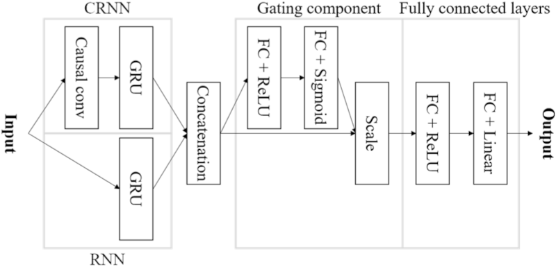
Schematic of the proposed model
1. Introduction
Time-series data exist in various aspects of daily life, such as electricity consumption, local temperatures, and road traffic volume. The forecasting of such data is important in a wide range of fields. For example, a cash conversion cycle can be used to improve financial efficiency by anticipating future demand and appropriately managing inventory. Similarly, traffic efficiency can be improved by understanding the ever-changing traffic congestion on roads and identifying appropriate routes. Various forecasting methods for time-series data have been proposed to address these requirements.
One of the most well-known time-series forecasting methods is the autoregressive integrated moving average (ARIMA) model 1. It is sufficiently flexible to include other types of time-series models such as autoregressive (AR), moving average, and autoregressive moving average (ARMA). However, ARIMA generally has difficulty capturing complex nonlinear patterns in time-series data, and selecting an appropriate model order can become computationally expensive when modeling long-term temporal dependencies. In contrast, feedforward neural networks (FNNs) can model nonlinear trends and uncertainty 2, but they require a larger sample size for accurate forecasts than statistical methods such as ARIMA. In addition, although FNNs effectively model patterns among samples, they generally have difficulty capturing long-term dependencies in the time-series direction. Against this background, deep neural networks (DNNs) have been intensively studied in artificial intelligence research and have had a significant impact on solving a wide range of problems. For example, recurrent neural networks (RNNs) are frequently used in time-series processing tasks, such as natural language processing and demand forecasting. In particular, the long short-term memory (LSTM) and gated recurrent unit (GRU) 3,4, both of which are RNN variants, have had practical applications in machine translation and speech recognition 5,6,7 as they process sequential data effectively. In recent years, convolutional neural networks (CNNs), which are widely used in the field of imaging, have been increasingly used for time-series predictions 8,9. CNNs are computationally inexpensive compared with RNNs because they often require fewer model parameters. Convolutions that access long-term historical data through stacked dilated causal convolution layers have also been investigated 10. Conventionally, CNNs and RNNs have been used separately for image recognition and time-series processing, respectively. However, many hybrid architectures that combine them within a single network have recently been proposed. A widely known approach is the convolutional recurrent neural network (CRNN), in which a signal propagates sequentially from the input layer through a CNN to an RNN 11,12,13,14. It preprocesses the input time-series data with a CNN to extract features from the data and then feeds the resulting output to an RNN. Thus, the CNN can extract short-term local dependencies in the time series, and the RNN can detect long-term dependencies. The CRNN has also been used in various applications, such as using a CNN to process input data such as image data, graphs, and spectrograms, and an RNN to predict sequential data 15,16,17.
Thus, combining the advantages of a CNN and an RNN can produce better results than the use of only an RNN. However, the CRNN in the existing literature is a single network in which the RNN does not process the original input data. Specifically, because of forward propagation, the original input to the model is processed by the CNN, and the processed data are then processed by the RNN.
Because the original data also contain valuable time-series information, processing the original data with the RNN may provide features that differ from those of a CRNN. Therefore, by combining the features obtained from both the CRNN and RNN models, we expect to improve the expressiveness of a model and achieve highly accurate predictions.
We propose a hybrid forecasting method using a CRNN and an RNN as a tool that can be implemented even at the field level and discuss its effectiveness. Inspired by the gating mechanism 18,19, the proposed model aims to utilize features properly by controlling the output of the feature vectors obtained from the two branches through a gating mechanism. Although various multi-branch neural networks, CNN–RNN hybrids, and attention/gating mechanisms have been discussed in recent literature, the primary technical aspects of the proposed model that distinguish it from existing deep-learning approaches are summarized as follows.
Parallel dual-branch architecture with raw sequences: Unlike conventional serial CRNNs or standard residual networks that filter data sequentially, our model employs a parallel dual-branch structure. The CRNN branch extracts short-term local dependencies, while the RNN branch simultaneously processes the original input sequence. This parallel design is expected to mitigate the loss of long-term dependency information, which often occurs during convolutional filtering and pooling in standard sequential models.
Customized squeeze-and-excitation (SE)-inspired gating design: To integrate the distinct features of the two branches, we introduce a specific gating mechanism inspired by the SE block 19. Unlike complex attention models, our customized gate dynamically evaluates and scales concatenated feature vectors. This enables the network to adaptively prioritize either short-term fluctuations or long-term trends, depending on the input context, thereby achieving high expressiveness.
Application to practical industrial forecasting: We validated the robustness of this architecture using highly volatile real-world industrial datasets (automotive manufacturing sales and energy sectors). The proposed model achieved superior forecasting accuracy for sudden transitions, demonstrating its high viability for deployment at the operational field level.
In forecasting experiments using multiple types of real-world time-series data, including case studies in the automotive and energy fields, the proposed model outperformed conventional methods substantially. In addition, a comprehensive ablation study and architectural survey were conducted to validate the structure of the proposed model.
The improvement in the demand forecasting accuracy addressed in this paper is closely related to sustainable value chain management in manufacturing. Sugimura et al. 20 proposed a demand forecasting system for wholesale markets to support production planning in plant factories, demonstrating that higher forecasting accuracy directly contributes to optimized production and shipping plans. Furthermore, Yonemoto and Suwa 21 experimentally demonstrated that task scheduling in manufacturing systems directly affects the energy efficiency of an entire factory, providing evidence of the cascading effect by which production planning optimization leads to reduced energy consumption. Shimomoto et al. 22 demonstrated that reducing energy consumption through manufacturing process optimization constitutes a concrete step toward achieving green transformation. Building on these previous studies, we expect the improvement in demand forecasting accuracy achieved by the proposed model to contribute to reduced energy consumption and environmental impacts in manufacturing processes through optimized production planning.
The remainder of this paper is organized as follows. Section 2 describes previous studies related to the proposed model. Section 3 describes the proposed model, and Section 4 details the experimental methodology. Section 5 reports the results of a comparison with existing baselines using actual time-series data and the evaluation results of the proposed model. Finally, Section 6 summarizes and concludes the paper.
2. Related Research
This section describes studies and approaches related to the proposed model.
2.1. Activation Function
The activation function is a nonlinear function in a neural network that transforms a value passed from one neuron to another. The most commonly used activation functions are sigmoid and hyperbolic tangent functions, expressed as follows:
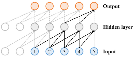
Fig. 1. Causal convolutions.
2.2. Causal Convolutions
Causal convolutions are designed to model time-series data without considering future steps 10, unlike the conventional convolutions commonly used in the imaging field (Fig. 1). Specifically, output \({\tilde{x}}_{t}\) at time \(t\) is designed to be independent of future inputs, beginning with \(x_{t+1}\).
2.3. Gated Recurrent Unit
The GRU is an extension of the vanilla RNN architecture and has a lower computational cost than LSTM 3,4, which is another gated RNN architecture, because it has fewer parameters and achieves comparable accuracy in some tasks 24. Let \(z_{t}\) and \(r_{t}\) be the update and reset gates at time \(t\), \(h_{t}\) be the output of the memory unit, and \({\tilde{h}}_{t}\) be the candidate value of the new hidden layer. Each is expressed as follows:
2.4. SE Network
The SE Network (SENet) won the ImageNet Large Scale Visual Recognition Challenge 2017 image-classification competition 19,25. The core of SENet is a mechanism called the SE block (Fig. 2). Its incorporation into any CNN model, such as VGG-16 26, the inception module 27, or ResNet 28, has been reported to improve performance over the original model. In the SE block, the 3D feature map (height, width, and channel) output by the convolutional layer is averaged over the spatial plane by global average pooling (GAP), converted into a channel-wise vector, and passed to a two-layer fully connected (FC) network. The FC layer computes the weighted sum of input vectors. Given an input signal \(X = \{x_1, x_2, \ldots, x_n\}\), the \(j\)-th output \(u_{j}\) of the FC layer is computed as follows:
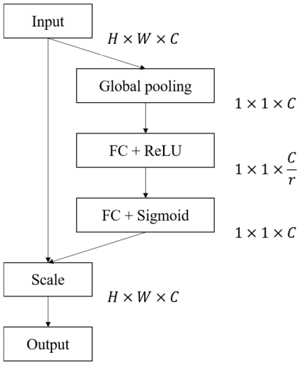
Fig. 2. SE block.
3. Proposed Model
Figure 3 presents an overview of the proposed model. In the proposed model, feature vectors obtained from two branches (CRNN and RNN) are passed through two FC layers before the output is controlled by a gating mechanism and the final prediction is produced.
3.1. CRNN and RNN
First, the input data are processed separately by the CRNN and RNN. In the CRNN branch, the causal convolutional layer (Conv1D: 16 filters, kernel size \(=6\), stride \(=1\), causal padding, dilation rate \(=1\), and ReLU activation) extracts short-term features of the time series, and its output is processed by a single-layer GRU (\(\tanh\) activation, return sequences = false). In contrast, the RNN branch processes the same raw input sequence directly through a single-layer GRU with the same configuration. The proposed model aims to enhance feature representation by appropriately utilizing the different feature vectors obtained from these two branches in the gating mechanism described below.
Specifically, the feature vector extracted from short-term patterns via the CRNN path and the feature vector capturing long-term dependencies from the raw sequence via the RNN path are integrated through a concatenation process. These two distinct vectors are concatenated along the feature dimension to construct a unified feature vector \(H = \{h_1, h_2, \ldots, h_c\}\), which is then passed as a single input to the subsequent gating mechanism.
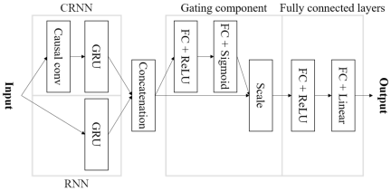
Fig. 3. Schematic of the proposed model.
3.2. Gate Mechanism
The feature vector outputs from each branch are connected and controlled by a gating mechanism. The gating mechanism controls the contribution of each feature vector to the final output. The gating mechanism of the proposed model is inspired by the SE block and consists of two FC layers 19, excluding GAP. The gated output \(\tilde{u}\) is obtained by applying the gating mechanism to the concatenated feature vector \(H=\{h_1, h_2, \ldots, h_c\}\) of the CRNN and RNN, as follows:
4. Comparison Experiments with Conventional Methods
This section describes the evaluation methods used in our experiments. In the experiment, six forecasting methods, including the proposed model, were evaluated using six benchmark datasets for time-series forecasting.
4.1. Comparison Methods
This section describes the forecasting methods used as baselines for comparison, all of which were designed for use at the field level. The comparison methods used were as follows:
-
・
AR model: A time-series model in which the current value is regressed on past values.
-
・
ARIMA model: A model that applies an ARMA model to the \(d\)-th-order differenced time series.
-
・
Holt–Winters model: This method extends exponential smoothing by incorporating the trend and seasonal components of the time series.
-
・
GRU: RNN based on GRU cells.
-
・
LSTM: RNN based on LSTM cells.
-
・
Proposed model: The model proposed in this paper.
The AR and ARIMA models are among the best known and most frequently used statistical methods. The Holt–Winters method, another popular statistical method, is often used because demand data typically include seasonality and trends that can be modeled. In recent years, the GRU and LSTM have been among the most popular machine learning methods for time-series forecasting.
These baselines were intentionally selected because they represent well-established, widely adopted, and practically feasible methods in industrial applications, which aligned with the practical focus of this study. While more complex forecasting architectures have recently emerged, they often require significantly larger computational resources, extensive memory, and prolonged training times, making them less suitable for real-time or resource-constrained industrial edge-computing environments. Therefore, this study focused on comparing our model against standard, highly practical benchmarks. Furthermore, to evaluate the specific contribution of parallel architecture compared to a standard sequential network, we evaluated a direct CRNN structure in our ablation study as the configuration without the RNN branch. To ensure a fair comparison, we configured all deep learning-based models (GRU, LSTM, and our variants) under the same protocol. The main hyperparameters (the number of hidden units, learning rate, batch size, and context length) were fixed in advance based on preliminary experiments and applied identically to all models, and the number of training epochs was selected by monitoring the validation loss for the Electricity (Client 1) dataset and the training loss for the others.
4.2. Indices
The following two traditional indicators were used to evaluate the accuracy of each forecasting method:
-
・
Relative squared error (RSE)
-
・
Relative absolute error (RAE)
| Data | Type | Period | Sample rate |
| Car | Sedan (Model A) | 2013/01/01–2019/10/31 | 1 month |
| SUV (Model B) | 2012/02/01–2019/08/31 | ||
| Electricity | Client 1 | 2012/01/01–2014/12/31 | 1 hour |
| Client 2 | 2012/01/01–2014/12/31 | ||
|
Solar- Energy |
Alabama | 2006/01/01–2006/12/31 | 20 minutes |
| Arizona | 2006/01/01–2006/12/31 |
4.3. Case Data
The data used in the experiment were as follows, as summarized in Table 1.
-
・
Car: Monthly car sales data for two car models over several years, provided by a Japanese automotive manufacturer. This dataset is proprietary and cannot be made publicly available due to confidentiality restrictions.
-
・
Electricity: Hourly electricity consumption data from 2012 to 2014 for two customers (Clients 1 and 2), obtained from the UCI Machine Learning Repository. This dataset is publicly available and may be used with appropriate attribution 29.
-
・
Solar-Energy: Solar energy output data recorded at 20-min intervals across multiple sites in Alabama and Arizona in 2006, obtained from the National Renewable Energy Laboratory 30. This dataset is publicly available and has been widely used in academic research on energy forecasting.
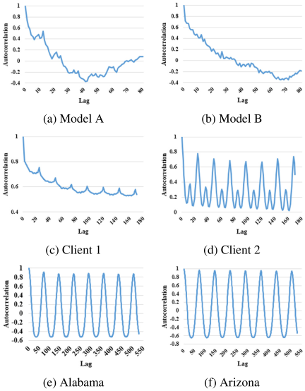
Fig. 4. Autocorrelation graphs for each data.
As shown in Table 1, the number of data points in these datasets differs substantially: the Car dataset contains 82 and 91 monthly observations for two car models, sedan (Model A) and SUV (Model B), respectively; the Electricity dataset contains 26,304 hourly observations per customer recorded from 2012 to 2014; and the Solar-Energy dataset contains 26,280 observations per site recorded at 20-min intervals during 2006. This difference reflects the inherent characteristics of each data source and is considered in the experimental design, particularly in the setting of recurrent layer units, which were set smaller for the Car dataset because of the limited sample size.
To examine the presence of long- and short-term repetitive cycles in the time-series data, Fig. 4 shows an autocorrelation graph for each dataset. Autocorrelation indicates the degree to which data are correlated with their past values and is defined as follows:
Figure 4 shows that Client 2, Alabama, and Arizona had repetitive cycles with high autocorrelation. In addition, Client 1 exhibited a repetitive cycle, although the autocorrelation becomes weaker over a longer period. However, the data without clear and consistent cycles may be more difficult to predict.
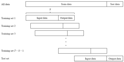
Fig. 5. Data preparation procedure for the proposed model.
4.4. Experimental Details
The forecast horizon for each dataset was set to 6, 24, and 72 for the Car, Electricity, and Solar-Energy datasets, respectively. This means that forecasts were made six months ahead for the Car data and one day ahead for the Electricity and Solar-Energy data. The input sequence length (context length) was set to \(\{6, 12\}\) for the Car data, and 48 and 72 for the Electricity and Solar-Energy data, respectively. The number of evaluation data points (test size) was set to four conditions \(\{24, 18, 12, 6\}\), and three independent trials were conducted for each condition. The number of units in the recurrent layer was set to a fixed value selected in advance for each dataset, selected from \(\{10, 25, 50, 100\}\) for the Car data and \(\{100, 200, 300\}\) for the Electricity and Solar-Energy data. The number of units in all FC layers was set to 1/2 of the recurrent layer units, and the number of epochs was limited to 300. The reduction ratio \(r\) was set to 4, considering the experimental environment of this study and the experiments of Hu et al. 19. Specifically, Hu et al. examined reduction ratios \(\{4, 8, 16, 32\}\) and reported that 16 was appropriate for SE-ResNet-50. However, because our model is relatively small, we set \(r=4\), which achieved the second-lowest top-five error after 16 in that study. The loss function was the mean squared error, and the Adam optimizer was used with default parameters (\(\mathit{lr}=0.001\), \(\beta_{1}=0.9\), \(\beta_{2}=0.999\), \(\epsilon=\textrm{1e-7}\)) 31. The batch size was set to 4, and min–max normalization (0–1 scaling) was applied to all input data. All the experiments were implemented using TensorFlow/Keras (Python 3.6). No early stopping was applied; instead, the model was saved every five epochs, and for each forecasting period, the checkpoint that minimized the validation loss (or the training loss where no validation set was used) was selected.
To clarify the evaluation process and chronological framework of the dataset, Fig. 5 depicts the data preparation procedure and the definition of the four forecasting periods utilized in our validation scheme. As shown in Fig. 5, the dataset was sequentially divided into training and test data to maintain temporal dependency, and the predictive performance was comprehensively evaluated across four independent forecasting periods (Periods 1–4). Accordingly, the values reported in Tables 2–4 represent the means and standard deviations calculated across four distinct periods. The standard deviation reflects the variability in the predictive performance across these forecasting periods, and because the number of evaluation periods is limited to four, it should be interpreted as a reference indicator of variability rather than a robust statistical measure.
| Data | Car | Electricity | Solar-Energy | ||||
| Type | Model A | Model B | Client 1 | Client 2 | Alabama | Arizona | |
| Methods | Metrics | ||||||
| AR | RSE | 2.405\(\pm\)2.08 | 1.432\(\pm\)0.34 | 0.999\(\pm\)0.70 | 0.406\(\pm\)0.48 | 0.1966\(\pm\)0.26 | 0.0076\(\pm\)0.01 |
| RAE | 1.459\(\pm\)0.87 | 1.152\(\pm\)0.09 | 0.994\(\pm\)0.29 | 0.517\(\pm\)0.44 | 0.0947\(\pm\)0.09 | 0.0555\(\pm\)0.02 | |
| ARIMA | RSE | 2.656\(\pm\)2.46 | 1.640\(\pm\)0.75 | 1.349\(\pm\)1.31 | 0.278\(\pm\)0.28 | 0.1790\(\pm\)0.28 | 0.0069\(\pm\)0.01 |
| RAE | 1.542\(\pm\)0.81 | 1.242\(\pm\)0.26 | 1.065\(\pm\)0.57 | 0.455\(\pm\)0.34 | 0.0722\(\pm\)0.04 | 0.0461\(\pm\)0.02 | |
| Holt–Winters | RSE | 2.840\(\pm\)1.66 | 3.457\(\pm\)2.19 | 0.843\(\pm\)0.44 | 0.536\(\pm\)0.43 | 0.7206\(\pm\)0.35 | 0.0884\(\pm\)0.06 |
| RAE | 1.599\(\pm\)0.46 | 1.794\(\pm\)0.58 | 1.034\(\pm\)0.33 | 0.656\(\pm\)0.22 | 0.3972\(\pm\)0.27 | 0.1701\(\pm\)0.08 | |
| GRU | RSE | 1.042\(\pm\)0.40 | 1.421\(\pm\)0.37 | 0.764\(\pm\)0.41 | 0.099\(\pm\)0.04 | 0.0396\(\pm\)0.04 | 0.0081\(\pm\)0.00 |
| RAE | 1.029\(\pm\)0.28 | 1.155\(\pm\)0.25 | 0.834\(\pm\)0.26 | 0.249\(\pm\)0.03 | 0.1155\(\pm\)0.07 | 0.0603\(\pm\)0.00 | |
| LSTM | RSE | 0.959\(\pm\)0.30 | 1.734\(\pm\)0.65 | 0.899\(\pm\)0.58 | 0.097\(\pm\)0.03 | 0.0392\(\pm\)0.05 | 0.0065\(\pm\)0.00 |
| RAE | 0.993\(\pm\)0.23 | 1.306\(\pm\)0.34 | 0.906\(\pm\)0.36 | 0.259\(\pm\)0.01 | 0.1129\(\pm\)0.08 | 0.0553\(\pm\)0.01 | |
| Proposed model | RSE | 0.781\(\pm\)0.36 | 1.212\(\pm\)0.44 | 0.523\(\pm\)0.31 | 0.076\(\pm\)0.05 | 0.0114\(\pm\)0.01 | 0.0053\(\pm\)0.00 |
| RAE | 0.858\(\pm\)0.30 | 1.030\(\pm\)0.17 | 0.735\(\pm\)0.16 | 0.223\(\pm\)0.04 | 0.0624\(\pm\)0.03 | 0.0467\(\pm\)0.01 | |
| Methods | Model A | Model B | Client 1 | Client 2 | Alabama | Arizona |
| AR | 0.478\(\pm\)0.45 | 0.086\(\pm\)0.19 | 0.510\(\pm\)0.37 | 0.926\(\pm\)0.04 | 0.9942\(\pm\)0.00 | 0.9990\(\pm\)0.00 |
| ARIMA | 0.001\(\pm\)0.60 | 0.075\(\pm\)0.39 | 0.547\(\pm\)0.37 | 0.953\(\pm\)0.04 | 0.9964\(\pm\)0.00 | 0.9991\(\pm\)0.00 |
| Holt–Winters | 0.507\(\pm\)0.25 | 0.377\(\pm\)0.17 | 0.616\(\pm\)0.20 | 0.862\(\pm\)0.13 | 0.8790\(\pm\)0.10 | 0.9701\(\pm\)0.01 |
| GRU | 0.425\(\pm\)0.48 | 0.600\(\pm\)0.26 | 0.397\(\pm\)0.42 | 0.956\(\pm\)0.02 | 0.9929\(\pm\)0.01 | 0.9967\(\pm\)0.00 |
| LSTM | 0.488\(\pm\)0.31 | 0.603\(\pm\)0.18 | 0.363\(\pm\)0.48 | 0.957\(\pm\)0.02 | 0.9872\(\pm\)0.01 | 0.9979\(\pm\)0.00 |
| Proposed model | 0.500\(\pm\)0.48 | 0.551\(\pm\)0.33 | 0.657\(\pm\)0.28 | 0.966\(\pm\)0.02 | 0.9962\(\pm\)0.00 | 0.9984\(\pm\)0.00 |
| Data | Car | Electricity | Solar-Energy | ||||
| Type | Model A | Model B | Client 1 | Client 2 | Alabama | Arizona | |
| Methods | Metrics | ||||||
|
Proposed model without CRNN |
RSE | 1.252\(\pm\)0.35 | 1.338\(\pm\)0.30 | 0.841\(\pm\)0.31 | 0.084\(\pm\)0.05 | 0.0183\(\pm\)0.02 | 0.0081\(\pm\)0.00 |
| RAE | 1.118\(\pm\)0.22 | 1.144\(\pm\)0.12 | 0.881\(\pm\)0.17 | 0.229\(\pm\)0.05 | 0.0783\(\pm\)0.04 | 0.0565\(\pm\)0.01 | |
|
Proposed model without RNN |
RSE | 1.007\(\pm\)0.21 | 1.422\(\pm\)0.27 | 0.738\(\pm\)0.29 | 0.088\(\pm\)0.06 | 0.0312\(\pm\)0.04 | 0.0055\(\pm\)0.00 |
| RAE | 1.027\(\pm\)0.20 | 1.163\(\pm\)0.22 | 0.782\(\pm\)0.12 | 0.224\(\pm\)0.06 | 0.1054\(\pm\)0.08 | 0.0499\(\pm\)0.01 | |
|
Proposed model without Gate |
RSE | 0.948\(\pm\)0.34 | 1.443\(\pm\)0.31 | 0.697\(\pm\)0.42 | 0.096\(\pm\)0.05 | 0.0387\(\pm\)0.04 | 0.0063\(\pm\)0.00 |
| RAE | 0.983\(\pm\)0.25 | 1.161\(\pm\)0.22 | 0.872\(\pm\)0.21 | 0.230\(\pm\)0.05 | 0.1068\(\pm\)0.07 | 0.0518\(\pm\)0.01 | |
| Proposed model | RSE | 0.781\(\pm\)0.36 | 1.212\(\pm\)0.44 | 0.523\(\pm\)0.31 | 0.076\(\pm\)0.05 | 0.0114\(\pm\)0.01 | 0.0053\(\pm\)0.00 |
| RAE | 0.858\(\pm\)0.30 | 1.030\(\pm\)0.17 | 0.735\(\pm\)0.16 | 0.223\(\pm\)0.04 | 0.0624\(\pm\)0.03 | 0.0467\(\pm\)0.01 | |
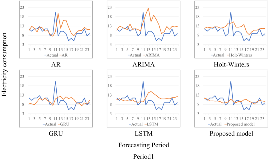
Fig. 6. Actual and predicted values for Client 1 in Forecasting Period 1.
5. Experimental Results and Discussion
5.1. Comparison Experiment
In Tables 2–4, each reported value represents the mean performance across the four forecasting periods (Periods 1–4), and the ± value denotes the standard deviation across these periods. Because the number of the forecasting periods was limited to four, this standard deviation should be interpreted as a reference indicator of variability rather than a robust statistical measure. Table 2 summarizes the evaluation results for each forecasting method. In addition, because the accuracy of time-series forecasting varies depending on the forecasting period, we conducted experiments for each of the four forecasting periods. Table 2 shows that the proposed model outperformed the conventional methods for most data and indicators. In particular, the proposed model substantially outperformed the conventional methods on the Client 1 data. Fig. 6 shows the evolution of the actual and predicted values of the data in question. These data were characterized by rapid changes in values over a short period; however, the proposed model was the most accurate in predicting these rapid transitions. However, most of the conventional methods exhibited a linear trend in the predicted values and failed to capture the characteristics of the actual values. Similar prediction trends were observed for Forecasting Periods 2–4. Appendix A presents detailed results for these periods. To compare the degree of similarity between the predicted and actual values, Table 3 shows the Pearson correlation coefficient (PCC) for each forecasting method. The PCC expresses the degree of the linear relationship between two variables. For two sets of data consisting of the actual values \(\boldsymbol{y} = (y_1, y_2, \ldots, y_n)\) and the predicted values \(\boldsymbol{\hat{y}} = (\hat{y}_1, \hat{y}_2, \ldots, \hat{y}_n)\), it is defined as follows:
| Methods | Model A | Model B | Client 1 | Client 2 | Alabama | Arizona |
| AR | 5 | 1 | 5 | 6 | 4 | 5 |
| ARIMA | 6 | 5 | 6 | 4 | 5 | 4 |
| Holt–Winters | 4 | 6 | 3 | 5 | 6 | 6 |
| GRU | 3 | 2 | 2 | 2 | 2 | 1 |
| LSTM | 1 | 4 | 4 | 1 | 3 | 2 |
| Proposed model | 2 | 3 | 1 | 3 | 1 | 3 |
Table 3 shows that, for Client 1, the proposed model had the highest value, which had the best approximation of the actual value. Client 2 also showed a high value for the proposed model, indicating that the proposed model consistently achieved high predictive accuracy across all evaluations.
For Alabama and Arizona, ARIMA yielded the highest values; however, the numerical difference between ARIMA and the proposed model was very small.
Statistical and DNN-based methods, including the proposed model, exhibited differences in the stability of their prediction accuracy. Table 5 lists the methods in ascending order of variance in their RSE values. Table 5 shows that the DNN-based methods obtained the highest rankings. Although Table 5 shows that the GRU achieved a slightly lower average rank (2.00) than the proposed model (2.17) across the six datasets, the actual RSE values in Table 2 reveal that the proposed model achieved competitive or superior accuracy in absolute terms on most datasets. In particular, the proposed model demonstrated substantially better performance on the Client 1 dataset, where accurate prediction of sudden value transitions was required. Therefore, considering both the ranking-based variance in Table 5 and the absolute error values in Table 2, the proposed model provides a favorable combination of predictive accuracy and stability.
Furthermore, Table 2 shows that better results were obtained for data with highly autocorrelated periodic patterns, as shown in Fig. 4. Specifically, the data were categorized in descending order of the numerical value of the evaluation index of each dataset as follows: Solar-Energy, Electricity (Client 2), Electricity (Client 1), and Car.
This indicates that to a certain extent, the difficulty in forecasting a time series can be estimated in advance by examining its autocorrelation.
5.2. Ablation Study
An ablation study was conducted to verify the necessity of each mechanism (CRNN, RNN, and gating mechanism) that constitutes the proposed model. Specifically, prediction experiments were conducted using a model with one mechanism removed from the proposed model, and the results were compared with those of the proposed model. The ablated models used were as follows:
-
・
Proposed model without CRNN: A model in which the CRNN branch is removed.
-
・
Proposed model without RNN: A model with the RNN branch removed.
-
・
Proposed model without gate: A model with the gate mechanism removed.
Table 4 summarizes the evaluation results for the ablated and proposed models. The proposed model performed better than the ablated models, which suggests that the configuration of the proposed model is more effective for higher prediction performance. No significant difference was observed between the evaluations of the proposed model without the CRNN and that without the RNN, indicating that the CRNN and RNN branches alone yielded comparable prediction performance.
In contrast, the full proposed model, which incorporates both components, achieved the best overall performance. Subsequently, we investigated the contribution of these two branches to forecasting in the proposed model, as described in the next section.
5.3. Investigation of Gate Output
We investigated the interaction of the CRNN and RNN branches when making predictions. Hence, we investigated the output vector of the gating mechanism when the test data were input into the trained models. Thus, we could determine the weight assigned to each branch. Specifically, because the output of the gating mechanism is activated by a sigmoid function, each vector element is mapped within a range of zero to one. This means that more important vectors are assigned larger weights, whereas unnecessary vectors are suppressed toward 0. Table 6 summarizes the average output vectors of the gates for each branch during each forecasting period.
Table 6 shows that, in all cases, the output of neither the CRNN nor the RNN branch was strongly suppressed, indicating that the feature vectors obtained from both branches contributed to improving the prediction. Furthermore, the RNN branch was occasionally weighted more heavily, which may have had a significant impact on the final prediction. Although the existing literature does not report that CRNNs consistently achieve better results than RNNs, our results suggest that the interaction between the CRNN and RNN branches can achieve better performance.
| Data | Car | |||||||||
| Type | Model A | Model B | ||||||||
| Period | Mean | Period | Mean | |||||||
| Method | 1 | 2 | 3 | 4 | 1 | 2 | 3 | 4 | ||
| CRNN | 0.534 | 0.550 | 0.583 | 0.540 | 0.552 | 0.521 | 0.510 | 0.506 | 0.507 | 0.511 |
| RNN | 0.552 | 0.524 | 0.520 | 0.526 | 0.531 | 0.510 | 0.518 | 0.505 | 0.504 | 0.509 |
| Data | Electricity | |||||||||
| Type | Client 1 | Client 2 | ||||||||
| Period | Mean | Period | Mean | |||||||
| Method | 1 | 2 | 3 | 4 | 1 | 2 | 3 | 4 | ||
| CRNN | 0.119 | 0.081 | 0.194 | 0.085 | 0.120 | 0.049 | 0.053 | 0.148 | 0.048 | 0.074 |
| RNN | 0.169 | 0.137 | 0.175 | 0.122 | 0.151 | 0.105 | 0.105 | 0.248 | 0.115 | 0.143 |
| Data | Solar-Energy | |||||||||
| Type | Alabama | Arizona | ||||||||
| Period | Mean | Period | Mean | |||||||
| Method | 1 | 2 | 3 | 4 | 1 | 2 | 3 | 4 | ||
| CRNN | 0.182 | 0.237 | 0.195 | 0.147 | 0.190 | 0.179 | 0.114 | 0.297 | 0.121 | 0.178 |
| RNN | 0.186 | 0.254 | 0.156 | 0.185 | 0.195 | 0.196 | 0.200 | 0.396 | 0.180 | 0.243 |
6. Conclusion
We propose a novel hybrid method for improving forecasting performance and evaluated it on multiple types of time-series datasets from the automotive and energy sectors. The proposed model comprises two branches (CRNN and RNN) and a gating mechanism. The gating mechanism controls the interactions between the feature vectors obtained from the two branches, thereby enabling the model to adaptively combine complementary information. The experimental results show that the proposed model outperforms conventional methods in forecasting experiments on multiple benchmark datasets. Given the large number of adjustable hyperparameters in the proposed model, future research should investigate the appropriate hyperparameter settings and evaluate their generalizability to larger benchmark datasets and multivariate time-series forecasting tasks.
- [1] G. E. Box and D. A. Pierce, “Distribution of residual autocorrelations in autoregressive-integrated moving average time series models,” J. Am. Stat. Assoc., Vol.65, No.332, pp. 1509-1526, 1970. https://doi.org/10.1080/01621459.1970.10481180
- [2] G. Zhang, B. E. Patuwo, and M. Y. Hu, “Forecasting with artificial neural networks: The state of the art,” Int. J. Forecast., Vol.14, No.1, pp. 35-62, 1998. https://doi.org/10.1016/S0169-2070(97)00044-7
- [3] S. Hochreiter and J. Schmidhuber, “Long short-term memory,” Neural Comput., Vol.9, No.8, pp. 1735-1780, 1997. https://doi.org/10.1162/neco.1997.9.8.1735
- [4] K. Cho, B. van Merriënboer, D. Bahdanau, and Y. Bengio, “On the properties of neural machine translation: Encoder-decoder approaches,” arXiv:1409.1259, 2014. https://doi.org/10.48550/arXiv.1409.1259
- [5] Y. Wu et al., “Google’s neural machine translation system: Bridging the gap between human and machine translation,” arXiv:1609.08144, 2016. https://doi.org/10.48550/arXiv.1609.08144
- [6] W. Xiong et al., “The Microsoft 2017 conversational speech recognition system,” IEEE Int. Conf. Acoust. Speech Signal Process. (ICASSP), pp. 5934-5938, 2018. https://doi.org/10.1109/ICASSP.2018.8461870
- [7] A. Abdallah, M. Kasem, M. A. Hamada, and S. Sdeek, “Automated question-answer medical model based on deep learning technology,” Proc. 6th Int. Conf. Eng. MIS, Article No.13, 2020. https://doi.org/10.1145/3410352.3410744
- [8] T. Y. Kim and S. B. Cho, “Predicting residential energy consumption using CNN-LSTM neural networks,” Energy, Vol.182, pp. 72-81, 2019. https://doi.org/10.1016/j.energy.2019.05.230
- [9] J. Dong and S. Liang, “Hybrid CNN-LSTM-GNN neural network for A-share stock prediction,” Entropy, Vol.27, No.8, Article No.881, 2025. https://doi.org/10.3390/e27080881
- [10] A. van den Oord et al., “WaveNet: A generative model for raw audio,” Proc. 9th ISCA Workshop Speech Synth. (SSW 9), p. 125, 2016.
- [11] Z. Zhang and Y. Dong, “Temperature forecasting via convolutional recurrent neural networks based on time-series data,” Complexity, Vol.2020, Article No.3536572, 2020. https://doi.org/10.1155/2020/3536572
- [12] M. Alhussein, K. Aurangzeb, and S. I. Haider, “Hybrid CNN-LSTM model for short-term individual household load forecasting,” IEEE Access, Vol.8, pp. 180544-180557, 2020. https://doi.org/10.1109/ACCESS.2020.3028281
- [13] A. Agga, A. Abbou, Y. El Houm, and M. Labbadi, “Short-term load forecasting based on CNN and LSTM deep neural networks,” IFAC-PapersOnLine, Vol.55, No.12, pp. 777-781, 2022. https://doi.org/10.1016/j.ifacol.2022.07.407
- [14] I. E. Livieris, E. Pintelas, and P. Pintelas, “A CNN–LSTM model for gold price time-series forecasting,” Neural Comput. Appl., Vol.32, pp. 17351-17360, 2020. https://doi.org/10.1007/s00521-020-04867-x
- [15] A. Lazcano, P. J. Herrera, and M. Monge, “A combined model based on recurrent neural networks and graph convolutional networks for financial time series forecasting,” Mathematics, Vol.11, No.1, Article No.224, 2023. https://doi.org/10.3390/math11010224
- [16] E. Çakır, G. Parascandolo, T. Heittola, H. Huttunen, and T. Virtanen, “Convolutional recurrent neural networks for polyphonic sound event detection,” IEEE/ACM Trans. Audio Speech Lang. Process., Vol.25, No.6, pp. 1291-1303, 2017. https://doi.org/10.1109/TASLP.2017.2690575
- [17] Y. Li, R. Yu, C. Shahabi, and Y. Liu, “Diffusion convolutional recurrent neural network: data-driven traffic forecasting,” Proc. Int. Conf. Learn. Represent. (ICLR), 2018.
- [18] R. K. Srivastava, K. Greff, and J. Schmidhuber, “Training very deep networks,” Adv. Neural Inf. Process. Syst. 28, 2015.
- [19] J. Hu, L. Shen, and G. Sun, “Squeeze-and-excitation networks,” Proc. IEEE Conf. Comput. Vis. Pattern Recognit. (CVPR), pp. 7132-7141, 2018. https://doi.org/10.1109/CVPR.2018.00745
- [20] N. Sugimura, N. Q. Thinh, S. Kohama, Y. Fukui, and K. Iwamura, “A study on demand forecasting of wholesale markets of lettuces for production planning in plant factories,” Int. J. Automation Technol., Vol.16, No.2, pp. 218-229, 2022. https://doi.org/10.20965/ijat.2022.p0218
- [21] R. Yonemoto and H. Suwa, “Task scheduling of material-handling manipulator for enhancing energy efficiency in flow-type FMS,” Int. J. Automation Technol., Vol.14, No.6, pp. 943-950, 2020. https://doi.org/10.20965/ijat.2020.p0943
- [22] K. Shimomoto, M. Nakamura, and T. Samukawa, “Energy consumption-oriented process design based on specific energy-consumption model,” Int. J. Automation Technol., Vol.20, No.1, pp. 24-37, 2026. https://doi.org/10.20965/ijat.2026.p0024
- [23] V. Nair and G. E. Hinton, “Rectified linear units improve restricted Boltzmann machines,” Proc. 27th Int. Conf. Mach. Learn. (ICML), 2010.
- [24] J. Chung, C. Gulcehre, K. Cho, and Y. Bengio, “Empirical evaluation of gated recurrent neural networks on sequence modeling,” arXiv:1412.3555, 2014. https://doi.org/10.48550/arXiv.1412.3555
- [25] O. Russakovsky et al., “ImageNet large-scale visual recognition challenge,” Int. J. Comput. Vis., Vol.115, pp. 211-252, 2015. https://doi.org/10.1007/s11263-015-0816-y
- [26] K. Simonyan and A. Zisserman, “Very deep convolutional networks for large-scale image recognition,” arXiv:1409.1556, 2014. https://doi.org/10.48550/arXiv.1409.1556
- [27] C. Szegedy et al., “Going deeper with convolutions,” Proc. IEEE Conf. Comput. Vis. Pattern Recognit. (CVPR), 2015. https://doi.org/10.1109/CVPR.2015.7298594
- [28] K. He, X. Zhang, S. Ren, and J. Sun, “Deep residual learning for image recognition,” Proc. IEEE Conf. Comput. Vis. Pattern Recognit. (CVPR), pp. 770-778, 2016. https://doi.org/10.1109/CVPR.2016.90
- [29] D. Dua and C. Graff, UCI Machine Learning Repository. http://archive.ics.uci.edu/ml [Accessed March 24, 2026]
- [30] Y. Zhang, “Solar power data for integration studies,” National Renewable Energy Laboratory. https://www.nrel.gov/grid/solar-power-data.html [Accessed March 24, 2026].
- [31] D. P. Kingma and J. Ba, “Adam: A method for stochastic optimization,” arXiv:1412.6980, 2014. https://doi.org/10.48550/arXiv.1412.6980
Appendix
Appendix A. Forecasting Results for Client 1 in Forecasting Periods 2–4
Figures 7–9 show the actual and predicted values for the Client 1 dataset in Forecasting Periods 2–4, respectively, obtained using each forecasting method (AR, ARIMA, Holt–Winters, GRU, LSTM, and the proposed model). As in Forecasting Period 1 (Fig. 6), the actual values in these periods include sudden, short-term peaks. In Forecasting Period 2 (Fig. 7), the proposed model captured the sharp peak in the actual values, as did the AR and ARIMA models. In Forecasting Period 3 (Fig. 8), most of the conventional methods produced nearly flat predictions around the peak, whereas the proposed model partially reproduced the sudden increase. In Forecasting Period 4 (Fig. 9), where the fluctuations were smaller, all methods followed the overall trend of the actual values. These results are consistent with the observations for Forecasting Period 1 discussed in Section 5.1.
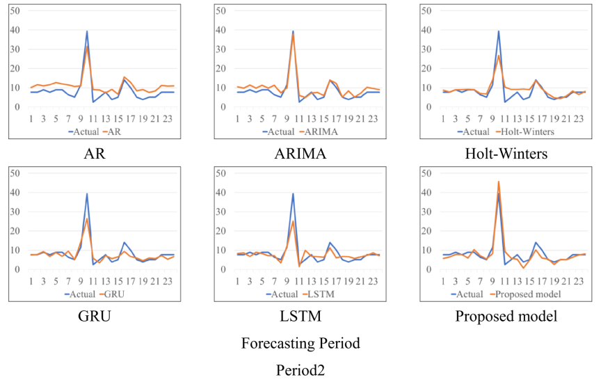
Fig. 7. Actual and predicted values for Client 1 in Forecasting Period 2.
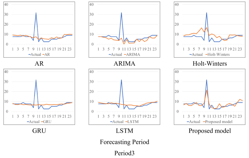
Fig. 8. Actual and predicted values for Client 1 in Forecasting Period 3.
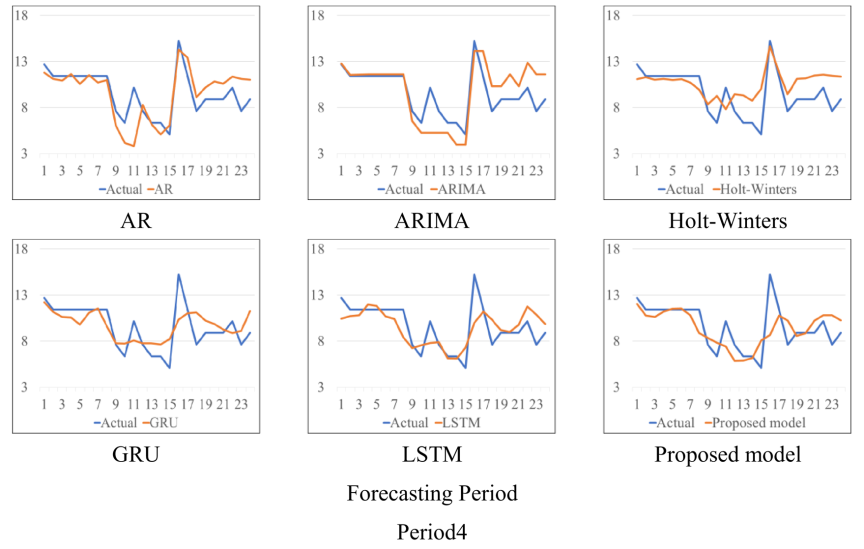
Fig. 9. Actual and predicted values for Client 1 in Forecasting Period 4.
This article is published under a Creative Commons Attribution-NoDerivatives 4.0 Internationa License.