
Research Paper:
Renewable-Energy-Based Global Supply Chain Network Design for Greenhouse Gas Reduction: A Comparison of Different Assembly Products
Tomoaki Takeda, Yuki Kinoshita†
 , and Tetsuo Yamada
Department of Informatics, The University of Electro-Communications
1-5-1 Chofugaoka, Chofu, Tokyo 182-8585, Japan
†Corresponding author

Greenhouse gas (GHG) emissions in global supply chains can be reduced by introducing renewable energy (RE) systems such as solar power generation systems. Some manufacturers commit themselves to the RE100 global initiative that encourages companies to source 100% of the electricity used in their business operations from RE. Thus, suppliers will face the risks of contract termination if suppliers fail to satisfy the target RE utilization rate to reduce GHG emissions. Besides costs, GHG emissions from electricity consumption during component production and GHG emissions from material production differ among suppliers due to differences in the availability of RE and regional energy mixes. Hence, in this study, we proposed a RE-based global supply chain network to reduce GHG emissions using an optimization model to satisfy the target RE utilization rate and GHG reduction rate simultaneously, where we considered the GHG emissions from electricity consumption and material production. In our model, the suppliers were allowed to purchase electricity generated by non-RE systems when they could not fulfill the electricity required to manufacture components from RE systems. We compared the RE utilization rate, GHG emissions, and total cost for two products (laptop and vacuum cleaner). We analyzed five scenarios for four countries (China, Malaysia, the United States, and Japan) where only one country implemented 100% RE, whereas the others installed 20-kW solar power generation systems and purchased additional electricity from non-RE providers. Both the laptops and vacuum cleaners exhibited a similar trend in terms of the GHG emissions and total cost.
1. Introduction
Owing to growing concerns over climate change driven by global warming as a result of the accumulation of greenhouse gases (GHGs) in the Earth’s atmosphere, there is a critical need to reduce GHG emissions such as carbon dioxide (CO\(_2\)) worldwide. Hence, the Government of Japan has declared its goal of achieving carbon neutrality by reducing net GHG emissions to zero by year 2050 1. To attain this goal, there is an urgent need to develop a carbon-neutral global supply chain network (GSCN). Assembled products such as laptops and home appliances are supplied through the GSCN, in which raw materials and components are manufactured across multiple countries based on an international division of labor, and subsequently distributed in markets worldwide with tariffs 2,3.
To reduce GHG emissions in the forward supply chain from sourcing to distribution, it is important to acknowledge that the GHG emissions from material production activities are significant 4. In addition, to achieve carbon neutrality, electrical power supplies used for production must transition from fossil fuel systems to renewable energy (RE) systems. For example, SHARP introduced photovoltaic systems in both foreign and domestic plants and achieved an RE rate of 25% in their electricity consumption 4. Moreover, to accelerate the use of RE systems, the RE100 was established as a global initiative to encourage companies to source 100% of the electricity used in their business operations from RE systems 5. Leading multinational corporations such as Microsoft in the United States and Panasonic in Japan have committed to this initiative 6,7. As a participant in the RE100 initiative, Seiko Epson has reportedly achieved its RE100 target through solar power generation and regionally aligned RE 8. GHG emissions in supply chains are categorized into three scopes 9. Scope 1 consists of direct emissions from sources owned by the corporation 9. Scope 2 comprises indirect emissions from purchased energy, steam, heating, or cooling 9. Scope 3 encompasses all other indirect emissions across the value chain 9. To attain carbon neutrality, manufacturers need to reduce GHG emissions across all scopes, and therefore, they require suppliers to reduce GHG emissions by using RE systems during component production. For example, Microsoft requires its major suppliers to use 100% RE 6. Apple also requires its suppliers to decarbonize all Apple-related operations by 2030 10. Therefore, to achieve RE100, suppliers are required to commit to the RE100 initiative in their production processes. This indicates that suppliers are at risk of having their contracts terminated by their clients if they do not fully commit to the RE100 initiative 11.
In addition to procurement costs, the GHG emissions from material production differ among suppliers due to differences in their energy mixes 12. Moreover, the amount of RE available is dependent on the supplier because of the different introduction rates of RE 13. Therefore, GHG emissions from electricity consumption and material production in the GSCN can be reduced by selecting suitable suppliers.
There are many papers on the GHG emissions of supply chain networks. Lo et al. 14 developed a multi-objective optimization model for a supply chain network to consider the operation costs, defect rates, sustainability performance, and risk of disruption using an augmented max–min approach in fuzzy multiple objective linear programming. They used a sustainability performance index to evaluate the supplier’s economic, environmental, and social aspects. However, they did not directly consider GHG emissions from material production or address the tariffs involved.
Eslamipoor and Sepehriyar 15 considered GHG emissions during transportation and energy consumption during the production of the final product. They developed mathematical models for a three-layer green supply chain network comprising suppliers, manufacturers, and sales centers to maximize profits under three carbon policies: carbon tax, carbon cap, and carbon trading. Although they addressed GHG emissions from energy consumption, they did not assess GHG emissions from material production, which generally constituted a significant amount of the total GHG emissions during production of the final product.
Nagao et al. 16 proposed an integer-programming model to design a GSCN based on the carbon border adjustment mechanism (CBAM), where they considered GHG emissions from material production, carbon taxes, and free trade agreements (FTAs) simultaneously. They also analyzed the effects of CBAM and carbon tax rates on factory location and supplier selection.
Edalatpour et al. 17 proposed an optimization model for a global sustainable closed-loop supply chain comprising suppliers, factories, distribution centers, markets, and recovery centers, where they integrated a set of rules called incoterms that defined the responsibilities of sellers and buyers in export transactions. They also considered the carbon pricing and advertisement costs. Although these studies considered GHG emissions and tariffs simultaneously, they did not consider GHG emissions from electricity consumption.
Based on the reviewed literature, it is apparent that previous studies have not simultaneously evaluated GHG emissions from material production and electricity consumption during component production. Furthermore, these studies did not consider contract termination for component supply if the RE utilization rate was not satisfied by the supplier.
Hence, in this study, we developed a GSCN, where we considered GHG emissions from electricity consumption during component production and GHG emissions from material production to achieve both RE utilization and GHG reduction rates. The GHG emissions from electricity consumption are dependent on the available and used amount of electricity for each supplier. Our model allowed suppliers to purchase electricity generated by external non-RE systems when the RE systems alone could not satisfy the electricity demand. Furthermore, when the suppliers could not meet the required RE utilization rate in keeping pace with their productivity, they could not supply the components due to contract termination.
The remainder of this paper is organized as follows. The GSCN based on a predetermined amount of RE and formulation of the mathematical model are described in Section 2. The input data and assumptions used in the numerical experiments are presented in Section 3. Sections 4 and 5 present the results for the laptop and vacuum cleaner, respectively. Finally, the conclusions drawn based on the key findings of this study are presented in Section 6, along with recommendations for future research.
2. Development of the GSCN Model
In this section, we describe our proposed model for a GSCN with GHG emissions from electricity consumption and material production. In our model, the amount of RE available for each supplier was set in advance as the input data.
2.1. GSCN Based on a Predetermined Amount of RE
The GSCN mathematical model is illustrated in Fig. 1. In this model, component \(j\) is produced by supplier \(o\) and is then transported to factory \(p\). The transported components \(j\) are then assembled into products at factory \(p\). Subsequently, the products are transported to market \(q\). We assumed that customs duties were imposed on international transportation.
However, tariffs were eliminated if there were FTAs between the countries involved in the supply chain. The GHG emissions arising from material production and electricity consumption by the suppliers were modeled and might be different among the suppliers. In addition, the amount of RE available differed among the suppliers, and these values were set as the input parameters for the model. The GSCN was constructed to satisfy both the GHG reduction and RE utilization rates set in advance. If the suppliers could not satisfy the required RE utilization rate, they could not provide the components because their contracts would be terminated.
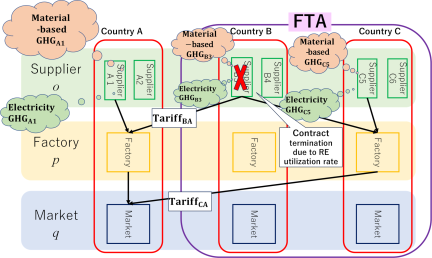
Fig. 1. GSCN model with GHG emissions from electricity consumption and material production.
2.2. Notations
The parameters used in the GSCN mathematical model are listed as follows.
-
I.
Sets
-
\(O\):
Set of suppliers, \(o\in O\)
-
\(P\):
Set of factories, \(p\in P\)
-
\(Q\):
Set of markets, \(q\in Q\)
-
\(J\):
Set of components, \(j\in J\)
-
\(O\):
-
II.
Decision variables
-
\(l_{oj}\):
Quantity of component \(j\) provided by supplier \(o\) [units]
-
\(v_{opj}\):
Quantity of component \(j\) transported from supplier \(o\) to factory \(p\) [units]
-
\(k_p\):
Quantity of products manufactured at factory \(p\) [units]
-
\(v_{pq}\):
Quantity of products transported from factory \(p\) to market \(q\) [units]
-
\(z_{pq}\):
Binary variable: 1 if a route between factory \(p\) and market \(q\) is open, 0 otherwise
-
\(u_p\):
Binary variable: 1 if factory \(p\) is open, 0 otherwise
-
\(l_{oj}\):
-
III.
Parameters
-
\(\mathit{TC}_{op}^{\mathit{PART}}\):
Transportation cost of component from supplier \(o\) to factory \(p\) [USD/unit]
-
\(\mathit{TC}_{pq}^{\mathit{PROD}}\):
Transportation cost of product from factory \(p\) to market \(q\) [USD/unit]
-
\(\mathit{PC}_{oj}\):
Procurement cost for component \(j\) at supplier \(o\) [USD/unit]
-
\(\mathit{CD}_{opj}^{\mathit{PART}}\):
Customs duty on component \(j\) from supplier \(o\) to factory \(p\)
-
\(\mathit{CD}_{pq}^{\mathit{PROD}}\):
Customs duty on a product from factory \(p\) to market \(q\)
-
\(\mathit{MC}_p\):
Manufacturing cost of a product at factory \(p\) [USD/unit]
-
\(\mathit{ORC}_{pq}\):
Fixed cost of opening a route between factory \(p\) and market \(q\) [USD]
-
\(\mathit{OFC}_p\):
Fixed cost of opening factory \(p\) [USD]
-
\(\mathit{EPC}_o\):
Electricity price per kWh at supplier \(o\) [USD/kWh]
-
\(N_j\):
Number of components \(j\) required per unit of product [units]
-
\(D_q\):
Product demand in market \(q\) [units]
-
\(\mathit{CAP}_p^{\mathit{PROD}}\):
Product manufacturing capacity at factory \(p\) [units]
-
\(\mathit{CAP}_{oj}^{\mathit{PART}}\):
Supply capacity for component \(j\) at supplier \(o\) [units]
-
\(\mathit{GHG}_{oj}^{\mathit{PART}}\):
GHG emissions from materials used in the production of component \(j\) at supplier \(o\) [g-CO\(_2\)eq/unit]
-
\(\mathit{GHG}_o^{\mathit{NREP}}\):
GHG emissions per kWh of nonrenewable electricity at supplier \(o\) [g-CO\(_2\)eq/kWh]
-
\(\mathit{TE}_{BL}\):
GHG emissions of the baseline case [g-CO\(_2\)eq]
-
\(\varepsilon\):
Rate of reduction of the total GHG emissions
-
\(\mathit{URE}_{oj}^{\mathit{CONS}}\):
Electricity consumption required to produce one unit of component \(j\) at supplier \(o\) [kWh/unit]
-
\(\mathit{URE}_{oj}^{\mathit{PUR}}\):
Electricity purchased to produce one unit of component \(j\) at supplier \(o\) [kWh/unit]
-
\(\alpha\):
Rate of utilization of RE in electricity consumption
-
\(\mathit{DISR}_o\):
1 if supplier \(o\) is terminated because it does not achieve the required rate of RE adoption, 0 otherwise
-
\(\mathit{OWRE}_o^{\mathit{GEN}}\):
Amount of RE that supplier \(o\) can generate from RE systems [kWh]
-
\(\mathit{PRRE}_o^{\mathit{CONS}}\):
Total electricity consumption required for component production of all manufacturable quantities at supplier \(o\) [kWh]
-
\(\mathit{PRRE}_o^{\mathit{PUR}}\):
Total purchased electricity required for component production of all manufacturable quantities at supplier \(o\) [kWh]
-
\(\gamma_o\):
Ratio of the total purchased electricity to the total consumed electricity at supplier \(o\)
-
\(M\):
Big M
-
\(\mathit{TC}_{op}^{\mathit{PART}}\):
-
IV.
Evaluation
-
\(\mathit{TC}\):
Total cost [USD]
-
\(\mathit{TPC}\):
Total component procurement cost [USD]
-
\(\mathit{TMC}\):
Total product manufacturing cost [USD]
-
\(\mathit{TTC}\):
Total transportation cost [USD]
-
\(\mathit{TRC}\):
Total cost to open routes [USD]
-
\(\mathit{TFC}\):
Total cost to open factories [USD]
-
\(\mathit{TAX}^{\mathit{PART}}\):
Total component duty cost [USD]
-
\(\mathit{TAX}^{\mathit{PROD}}\):
Total product duty cost [USD]
-
\(\mathit{TEC}\):
Total cost of electricity purchased [USD]
-
\(\mathit{TE}\):
Total GHG emissions [g-CO\(_2\)eq]
-
\(\mathit{TME}\):
Total GHG emissions from material production [g-CO\(_2\)eq]
-
\(\mathit{TRE}\):
Total GHG emissions from nonrenewable electricity consumption during component production [g-CO\(_2\)eq]
-
\(\mathit{TC}\):
2.3. Formulation
Equation (1) is an objective function that minimizes the total cost, which includes the procurement costs for components, the costs of manufacturing the product, transportation costs, the costs of establishing shipping routes, the costs of opening factories, the customs duties imposed on the components and products, and the purchasing costs of electricity by the suppliers.
Equation (2) represents the total GHG emissions in the production process, which is calculated as the sum of the GHG emissions from material production and electricity consumption. In Eq. (3), \(\varepsilon\) denotes the rate of GHG emissions reduction relative to the total GHG emissions. Thus, a supply chain configuration that achieves the target reduction can be determined by varying \(\varepsilon\).
Equations (4)–(11) represent the various cost components. Eq. (4) calculates the total procurement cost of the components, Eq. (5) calculates the total cost of manufacturing the product, Eq. (6) determines the total transportation cost, Eq. (7) determines the total cost of establishing shipping routes, Eq. (8) calculates the total cost of opening factories, and Eqs. (9) and (10) calculate the total customs duties of the components and products, respectively. Eq. (11) represents the total cost of electricity purchased by the suppliers.
Equations (12) and (13) calculate the GHG emissions from the materials used and electricity consumed during component production, respectively.
Equations (14)–(21) represent the constraints related to transportation. Components are purchased only from suppliers that satisfy the required RE utilization rate, as shown in Eq. (15).
Equations (22)–(26) are the constraints imposed on electricity. Eq. (22) represents the total electricity consumption required by the supplier to produce all manufacturable components. The reason for using the suppliers’ maximum production capacities in Eq. (22) is to ensure that the targeted RE utilization rate is satisfied by all suppliers. To achieve carbon neutrality, manufacturers are required to grasp all GHG emissions through the GSCN and they have to offset their GHG emissions (including energy consumption) by purchasing tradeable permits such as carbon credits and carbon emission allowances. This requirement regulates the underreporting of GHG emissions. Hence, manufacturers should have a margin of GHG emissions based on the maximum production capacity rather than based on the actual production quantity. In addition, the margin acts as a buffer against changes in the available amount of RE and the order quantities for each supplier. Eq. (23) indicates that the contract is terminated if a supplier’s total in-house RE generation does not satisfy the required RE utilization rate \(\alpha\). When a contract is terminated, the parameter \(\mathit{DISR}_o\) is set to 1. Eq. (24) defines the amount of electricity purchased by the supplier to produce all manufacturable quantities of components, which becomes zero when the in-house RE generation exceeds the total electricity consumption. In Eq. (25), \(\gamma_o\) denotes the ratio of the total electricity purchased by the supplier to the total electricity consumed. By using this ratio \(\gamma_o\), Eq. (26) calculates the amount of electricity that must be purchased by the supplier to produce a single component.
3. Input Data and Assumptions
The GHG emissions from electricity consumption and the purchasing price of electricity from non-RE providers were dependent on the suppliers. Table 1 shows the production costs for each country. The non-RE purchasing prices per 1 kWh for suppliers in China, Malaysia, the United States, and Japan were USD 0.087, 0.129, 0.145, and 0.176, respectively. In addition, the GHG emissions from electricity consumption from non-RE systems for suppliers in China, Malaysia, the United States, and Japan were 660.8, 614.6, 374.6, and 457.7 g-CO\(_2\)eq/kWh, respectively. The cost of manufacturing a given product varied depending on the country in which it was produced, as shown in Table 1.
| Factory |
Manufacturing cost of laptop [USD] |
Manufacturing cost of vacuum cleaner [USD] |
Opening factory cost [USD] |
Transportation cost [USD] (to Seattle) |
Opening route cost [USD] (to Seattle) |
| Shanghai | 3.5 | 2.50 | 76.0 | 0.9200 | 166.7 |
| Kuala Lumpur | 4.0 | 2.20 | 67.7 | 1.2900 | 166.7 |
| Seattle | 7.5 | 4.70 | 130.3 | 0.0001 | 166.7 |
| Tokyo | 10.1 | 6.33 | 179.9 | 0.7700 | 166.7 |
We selected a laptop and vacuum cleaner comprising 34 and 23 separate components, respectively, as the example products. Tables 2 and 3 show the GHG emissions from the materials used during production as well as the procurement costs. It is worth noting that the procurement of component #19 (motor) for the vacuum cleaner was excluded from the numerical experiments because it accounted for \(\sim\)95% of the total GHG emissions, as highlighted by Kotegawa et al. 12.
| Component No. | Component | Material type | Required quantity for one product | Weight [g] | Electricity consumption [kWh] | Procurement cost [USD] | GHG emission [g-CO\(_2\)eq] | ||||||
| China | Malaysia | The U.S. | Japan | China | Malaysia | The U.S. | Japan | ||||||
| 1 | Lithium ion battery | ABS | 1 | 305 | 8.24 | 0.532 | 0.485 | 0.597 | 0.934 | 3764.50 | 1623.81 | 715.73 | 715.90 |
| 2 | Key + top cover | PC/ABS | 1 | 51 | 1.38 | 0.089 | 0.081 | 0.100 | 0.156 | 629.47 | 271.52 | 119.68 | 119.71 |
| 3 | Membrane plug board | PET | 1 | 11 | 0.30 | 0.016 | 0.014 | 0.018 | 0.028 | 111.52 | 48.10 | 21.20 | 21.21 |
| 4 | Back plate | Al/Al alloy | 1 | 32 | 0.52 | 0.050 | 0.046 | 0.056 | 0.088 | 352.88 | 62.69 | 55.42 | 40.80 |
| 5 | Stabilizer | SUS (magnetic) | 1 | 3 | 0.08 | 0.003 | 0.002 | 0.003 | 0.005 | 23.36 | 6.29 | 3.92 | 3.30 |
| 6 | HDD | Al/Al alloy | 1 | 111 | 1.82 | 0.174 | 0.158 | 0.195 | 0.304 | 1224.05 | 217.47 | 192.24 | 141.51 |
| 7 | RAM | Epoxy resin | 1 | 14 | 0.38 | 0.036 | 0.032 | 0.040 | 0.062 | 251.56 | 108.51 | 47.83 | 47.84 |
| 8 | Case body | Al/Al alloy | 1 | 49 | 0.80 | 0.077 | 0.070 | 0.086 | 0.134 | 540.35 | 96.00 | 84.86 | 62.47 |
| 9 | Case body | Al/Al alloy | 1 | 8 | 0.13 | 0.013 | 0.011 | 0.014 | 0.022 | 88.22 | 15.67 | 13.86 | 10.20 |
| 10 | Case body + board + cord | SUS (magnetic) | 1 | 52 | 1.33 | 0.045 | 0.041 | 0.050 | 0.079 | 404.95 | 109.07 | 67.88 | 57.19 |
| 11 | Case body | ABS | 1 | 26 | 0.70 | 0.045 | 0.041 | 0.051 | 0.080 | 320.91 | 138.42 | 61.01 | 61.03 |
| 12 | Pad part | PC/ABS | 1 | 16 | 0.43 | 0.028 | 0.025 | 0.031 | 0.049 | 197.48 | 85.18 | 37.55 | 37.56 |
| 13 | Board component | Circuit board | 1 | 15 | 0.21 | 1.500 | 1.369 | 1.685 | 2.632 | 4311.20 | 1150.46 | 577.35 | 1052.59 |
| 14 | CPU | Circuit board | 1 | 7 | 0.10 | 1.500 | 1.369 | 1.685 | 2.632 | 4311.20 | 1150.46 | 577.35 | 1052.59 |
| 15 | Top cover | PC/ABS | 1 | 104 | 2.81 | 0.181 | 0.166 | 0.204 | 0.318 | 1283.63 | 553.69 | 244.05 | 244.11 |
| 16 | Top cover | SUS (magnetic) | 1 | 193 | 4.94 | 0.166 | 0.152 | 0.187 | 0.292 | 1503.00 | 404.83 | 251.96 | 212.25 |
| 17 | Bottom cover | PC/ABS | 1 | 177 | 4.78 | 0.309 | 0.282 | 0.347 | 0.542 | 2184.64 | 942.34 | 415.36 | 415.46 |
| 18 | Bottom cover | PC/ABS | 1 | 18 | 0.49 | 0.031 | 0.029 | 0.035 | 0.055 | 222.17 | 95.83 | 42.24 | 42.25 |
| 19 | Resin frame | PC/ABS | 1 | 5 | 0.14 | 0.009 | 0.008 | 0.010 | 0.015 | 61.71 | 26.62 | 11.73 | 11.74 |
| 20 | Metal frame | SUS (magnetic) | 1 | 28 | 0.72 | 0.024 | 0.022 | 0.027 | 0.042 | 218.05 | 58.73 | 36.55 | 30.79 |
| 21 | Fan | PC/ABS | 1 | 7 | 0.11 | 0.012 | 0.011 | 0.014 | 0.021 | 86.15 | 15.31 | 13.53 | 9.96 |
| 22 | Heat sink | Cu/Cu alloy | 1 | 63 | 1.03 | 0.258 | 0.235 | 0.289 | 0.452 | 1817.80 | 322.96 | 285.49 | 210.16 |
| 23 | Liquid crystal module | Glass | 1 | 425 | 4.72 | 4.860 | 4.434 | 5.457 | 8.526 | 12125.43 | 3432.15 | 2206.50 | 2646.62 |
| 24 | Front cover | Glass | 1 | 242 | 5.23 | 1.416 | 1.292 | 1.590 | 2.485 | 10696.24 | 3021.71 | 1571.43 | 1525.15 |
| 25 | Rear cover | PC/ABS | 1 | 233 | 6.29 | 0.406 | 0.371 | 0.456 | 0.713 | 2875.83 | 1240.49 | 546.77 | 546.90 |
| 26 | Connecting cable | Cu/Cu alloy | 1 | 7 | 0.11 | 0.029 | 0.026 | 0.032 | 0.050 | 201.98 | 35.88 | 31.72 | 23.35 |
| 27 | Antenna cable | Cu/Cu alloy | 1 | 5 | 0.08 | 0.020 | 0.019 | 0.023 | 0.036 | 144.27 | 25.63 | 22.66 | 16.68 |
| 28 | Frame | SUS (magnetic) | 1 | 59 | 1.51 | 0.051 | 0.046 | 0.057 | 0.089 | 459.47 | 123.76 | 77.02 | 64.88 |
| 29 | Web camera + board | Circuit board | 1 | 7 | 0.10 | 1.500 | 1.369 | 1.685 | 2.632 | 4311.20 | 1150.46 | 577.35 | 1052.59 |
| 30 | Motherboard | Circuit board | 1 | 171 | 2.41 | 1.500 | 1.369 | 1.685 | 2.632 | 4311.20 | 1150.46 | 577.35 | 1052.59 |
| 31 | Cushioning | Polyurethane | 1 | 3 | 0.05 | 0.009 | 0.008 | 0.010 | 0.015 | 37.85 | 14.91 | 7.86 | 7.03 |
| 32 | Speaker | PC/ABS | 1 | 30 | 0.81 | 0.052 | 0.048 | 0.059 | 0.092 | 370.28 | 159.72 | 70.40 | 70.42 |
| 33 | Wireless LAN card | Circuit board | 1 | 4 | 0.06 | 1.500 | 1.369 | 1.685 | 2.632 | 4311.20 | 1150.46 | 577.35 | 1052.59 |
| 34 | Cords | Cu/Cu alloy | 1 | 6 | 0.10 | 0.025 | 0.022 | 0.028 | 0.043 | 173.12 | 30.76 | 27.19 | 20.02 |
Note: ABS, acrylonitrile butadiene styrene; PC, polycarbonate; SUS, steel use stainless; HDD, hard disk drive; RAM, random access memory; LAN, local area network.
| Component No. | Component | Material type | Required quantity for one product | Weight [g] | Electricity consumption [kWh] | Procurement cost [USD] | GHG emission [g-CO\(_2\)eq] | ||||||
| China | Malaysia | The U.S. | Japan | China | Malaysia | The U.S. | Japan | ||||||
| 1 | Wheel | Polypropylene | 2 | 7 | 0.19 | 0.006 | 0.005 | 0.006 | 0.010 | 39.82 | 17.16 | 7.48 | 7.51 |
| 2 | Wheel stopper | Polypropylene | 2 | 2 | 0.05 | 0.001 | 0.001 | 0.002 | 0.002 | 9.63 | 4.15 | 1.81 | 1.82 |
| 3 | Upper nozzle | Polypropylene | 1 | 50 | 1.36 | 0.040 | 0.037 | 0.044 | 0.070 | 283.59 | 122.20 | 53.25 | 53.51 |
| 4 | Lower nozzle | Polypropylene | 1 | 41 | 1.11 | 0.033 | 0.030 | 0.036 | 0.057 | 232.33 | 100.11 | 43.62 | 43.84 |
| 5 | Nozzle | Polypropylene | 1 | 35 | 0.93 | 0.027 | 0.025 | 0.030 | 0.048 | 194.31 | 83.73 | 36.49 | 36.67 |
| 6 | Right handle | Polypropylene | 1 | 49 | 1.32 | 0.039 | 0.036 | 0.043 | 0.068 | 275.59 | 118.75 | 51.75 | 52.00 |
| 7 | Switch | Polyvinyl chloride | 1 | 5 | 0.13 | 0.003 | 0.003 | 0.004 | 0.006 | 23.65 | 10.19 | 4.44 | 4.46 |
| 8 | Left handle | Polypropylene | 1 | 52 | 1.40 | 0.041 | 0.038 | 0.046 | 0.072 | 291.19 | 125.47 | 54.67 | 54.95 |
| 9 | Left body | Polypropylene | 1 | 187 | 5.06 | 0.149 | 0.136 | 0.165 | 0.260 | 1054.76 | 454.50 | 198.05 | 199.02 |
| 10 | Right body | Polypropylene | 1 | 180 | 4.86 | 0.143 | 0.131 | 0.159 | 0.249 | 1013.13 | 436.56 | 190.23 | 191.17 |
| 11 | Dust case cover | Methacrylic resin | 1 | 37 | 0.99 | 0.055 | 0.050 | 0.061 | 0.096 | 391.89 | 168.87 | 73.58 | 73.95 |
| 12 | Mesh filter | Carbon fiber | 1 | 18 | 0.48 | 0.344 | 0.314 | 0.382 | 0.599 | 2967.54 | 1211.26 | 557.95 | 438.22 |
| 13 | Connection pipe | Aluminum alloy | 1 | 47 | 0.77 | 0.058 | 0.053 | 0.064 | 0.101 | 409.95 | 72.76 | 63.58 | 47.03 |
| 14 | Dust case | Methacrylic resin | 1 | 176 | 4.74 | 0.266 | 0.243 | 0.295 | 0.463 | 1882.72 | 811.27 | 353.51 | 355.25 |
| 15 | Exhaust tube | Polyvinyl chloride | 1 | 32 | 0.87 | 0.023 | 0.021 | 0.026 | 0.040 | 162.99 | 70.23 | 30.60 | 30.76 |
| 16 | Upper filter | Carbon fiber | 1 | 18 | 0.46 | 0.331 | 0.302 | 0.367 | 0.576 | 2853.34 | 1164.65 | 536.47 | 421.36 |
| 17 | Lower filter | Polypropylene | 1 | 29 | 0.79 | 0.023 | 0.021 | 0.026 | 0.041 | 165.19 | 71.18 | 31.02 | 31.17 |
| 18 | Protection cap | Polystyrene | 1 | 22 | 0.60 | 0.025 | 0.023 | 0.028 | 0.044 | 177.60 | 76.53 | 33.35 | 33.51 |
| 20 | Rubber of outer frame of fan | Synthetic rubber | 1 | 23 | 0.81 | 0.032 | 0.029 | 0.035 | 0.056 | 332.83 | 125.15 | 65.88 | 55.96 |
| 21 | Outer frame of fan | Aluminum alloy | 1 | 55 | 0.90 | 0.068 | 0.062 | 0.075 | 0.118 | 478.96 | 85.01 | 74.29 | 54.94 |
| 22 | Lower fan | Polypropylene | 1 | 15 | 0.41 | 0.012 | 0.011 | 0.013 | 0.021 | 84.93 | 36.60 | 15.95 | 16.03 |
| 23 | Fan | Aluminum alloy | 1 | 62 | 1.02 | 0.077 | 0.070 | 0.085 | 0.133 | 539.71 | 95.79 | 83.71 | 61.91 |
The procurement costs and GHG emissions from material production were calculated based on the work of Yoshizaki et al. 18 and the Life Cycle Inventory (LCI) database incorporating Asian I/O tables 19. The electricity consumption was calculated based on the work of Nagai 11. The manufacturing costs of laptops and vacuum cleaners were estimated using the assembly and reliability evaluation method 20,21. The factory opening and transportation costs were calculated based on the international price level index 22 and transportation distance, respectively.
First, the procurement cost of each component was calculated. One representative material was identified for each component. The material price per gram [USD/g] was estimated using the Census of Manufacture 23, weight, and the international price level index 22. The procurement cost for each country was determined using the following equation:
Second, the GHG emissions from material production were calculated using the procurement costs and LCI database incorporating Asian I/O tables 19 by matching the material type and intensity of the GHG emissions. It shall be noted that the variations in GHG emissions from material production among the countries were attributed to their respective energy mixes 19.
Finally, the electricity consumption for each component was calculated based on the electricity consumption during material processing 24 and the proportion of Japanese GHG emissions intensities in the LCI database incorporating Asian I/O tables 19. Nagai 11 assumed that the electricity consumption for 1 kg of polypropylene production was 27 kWh based on the work of Takatori 24. The electricity consumption of each component was estimated using the proportions of weight and Japanese GHG emissions intensities corresponding to the material type of the component.
The supply chain network comprised four countries: China, Malaysia, the United States, and Japan. Each country was assumed to have 13 supplier locations and a single factory location. We selected Seattle in the United States as the market, and the number of products in demand was set to 24,000 units. The supply capacity of each component was set as the number of components necessary to meet the total product demand of the market. The production capacity of each factory was set to 12,000 units. The Trans-Pacific Partnership (TPP) was regarded as the FTA. The customs duties were defined as follows: 25% between the United States and China, 10% between a TPP member and nonmember, and 0% among TPP members. Malaysia and Japan were designated as members of an FTA. The electricity data provided by Nagai 11 were used for the solar panels. Furthermore, based on the work of Nagai 11, the system output coefficient was set to 0.75, the solar panel generation capacity was assumed to be 20 kW, and the standard solar irradiance was set to 1 kW/m\(^2\).
Numerical experiments were conducted for five scenarios. One was a “non-adoption” scenario in which none of the four countries had installed photovoltaic modules, and the suppliers purchased all the nonrenewable electricity required to manufacture the components from the grid. Another was the “advanced” scenario in which one country could cover 100% of the RE required by the supplier to manufacture the components. In contrast, for the other three countries, the suppliers installed panels with a generation capacity of 20 kW and purchased their remaining electricity from the grid. The RE utilization rate was varied from 0.0 to 1.0 with 0.1 intervals in all advanced scenarios. All experiments were conducted using Nuorium Optimizer optimization software 25 on a laptop with an Intel® Core™ i7-10710U central processing unit with a clock rate of 1.10 GHz on Windows 11 Pro operating system.
4. Analysis for Laptops
In this analysis, we identified that the laptop components used hybrid integrated circuits as the raw materials, specifically the circuit board unit, central processing unit, web camera, motherboard, and wireless LAN card (components #13, #14, #29, #30, and #33) and those that used liquid crystal display modules (component #23) were characterized by high costs and large GHG emissions, as shown in Table 2. Based on these characteristics, the GHG emissions and total cost for the different scenarios are discussed in this section.
4.1. Trends of GHG Emissions and Total Cost for Laptop Production
The baseline GHG emissions were defined as the values at an RE utilization rate of \(\alpha=0\) and GHG reduction rate of \(\varepsilon=0\) in each scenario. In this study, “high cost-effectiveness” refers to a state in which the GHG emissions are reduced while the increase in the total cost is suppressed. In Fig. 2, the point immediately before the slope changed drastically in the set of Pareto-optimal solutions was defined as a situation with excellent cost-effectiveness because attempting to reduce GHG emissions beyond this point would require a substantial increase in the total cost. The total GHG emissions and total cost for the five scenarios are shown in Fig. 2. It shall be noted that the scales of the axes in each graph differ from one another.
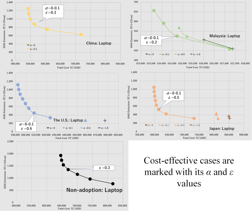
Fig. 2. Relationships between the GHG emissions and total cost for laptop production.
Figure 2 shows the total cost and GHG emissions for each RE utilization rate and GHG reduction rate. It shall be highlighted that only the results for \(\alpha=0.0\), 0.1, 0.5, and 1.0 are shown in Fig. 2 because the other results overlap with them. We present the detailed results in Appendix A. Each RE utilization rate was highlighted using a different color. Although the RE utilization and GHG reduction rates might be similar constraints for GHG reduction, they sometimes conflicted with one another.
For example, a higher RE utilization rate could regulate changes in suppliers in countries that achieve RE100; however, the suppliers must be switched to satisfy the higher GHG reduction rates. However, these requirements resulted in infeasible solutions. Therefore, the combination of RE utilization and GHG reduction rates required to obtain a feasible solution was dependent on the scenario.
As shown in Fig. 2, in the non-adoption scenario, the GHG emissions could be reduced by changing the configuration of suppliers, even without introducing RE facilities. The minimum GHG emissions were obtained at a GHG reduction rate of \(\varepsilon=0.6\) and total cost of USD 816,877. However, the total cost increased proportionally with this reduction. In particular, the increase in the total cost became significant when the GHG reduction rate was set to a value greater than 0.3.
When the GHG reduction rate was \(\varepsilon=0.0\)–0.4, Chinese and Malaysian factories were opened in the China advanced scenario. When \(\varepsilon=0.5\), a factory was opened in the United States instead of in China. Furthermore, in this scenario, the results confirmed that setting a high RE utilization rate \(\alpha\) led to no feasible solutions. The factors contributing to this were rooted in the baseline (\(\alpha=0\), \(\varepsilon=0\)) in which the GHG emissions from material production accounted for \(\sim\)95.7% of the total GHG emissions due to Chinese suppliers complying with the RE100 initiative. Although some components were manufactured in Malaysia in the baseline case, many Chinese suppliers with RE100 facilities were selected for the baseline case. However, selecting suppliers in the United States or Japan would be effective to reduce GHG emissions from material production because these suppliers had lower GHG emissions in this regard.
It shall be noted that switching suppliers from China to the United States or Japan would reduce the ratio of suppliers located in China, which would reduce the RE utilization rate \(\alpha\) of the entire system. Thus, selecting Chinese suppliers was necessary to increase \(\alpha\); however, selecting non-Chinese suppliers was necessary to reduce GHG emissions from material production. In addition, increasing the proportion of Chinese suppliers increased the GHG emissions from material production, which could have caused the total GHG emissions to exceed the baseline value. Due to these conflicting conditions, only RE utilization rates of \(\alpha=0\) and 0.1 could be obtained for the China advanced scenario.
The baseline GHG emissions for the Malaysia advanced scenario were the lowest compared with those of all other scenarios. Consequently, it was difficult to reduce GHG emissions in this scenario if the RE utilization rate \(\alpha\) was set to a high value, and we could not obtain any feasible solutions.
In the baseline case (\(\alpha=0\), \(\varepsilon=0\)), the GHG emissions from material production accounted for \(\sim\)98.5% of the total GHG emissions. At this point, it was possible to reduce the GHG emissions by shifting suppliers to Malaysia, the United States, or Japan because some Chinese suppliers had already been selected. However, increasing the ratio of suppliers in the United States or Japan to further reduce the GHG emissions decreased the ratio of RE, which made it impossible to satisfy high \(\alpha\) constraints as in the China advanced scenario.
Meanwhile, we did not observe a significant increase in the total cost when the GHG emissions were reduced. This was indeed expected because a supplier configuration centered on Malaysia was selected as a relatively inexpensive producer, regardless of the location of the assembly factory. In addition, the reduction in the GHG emissions involved switching from Chinese to Malaysian suppliers for many components, which suppressed the increase in the total cost. It shall be noted that for \(\alpha\geq 0.9\), the supplier configuration did not change regardless of the GHG reduction rate.
In the United States advanced scenario, a factory was opened in the United States instead of in China when the rate of GHG reduction was set to \(\geq 70\)%, or when the RE utilization rate was set to \(\geq 20\)%. Although the total cost increased due to the relatively high cost of electricity in the United States, the reduction in GHG emissions was pronounced, where the GHG emissions decreased by up to \(\sim\)70% of the baseline values. This was likely because although procurement from China and Malaysia resulted in high baseline GHG emissions, shifting these suppliers to the United States or Japan could significantly reduce the GHG emissions. However, the total cost increased because the United States and Japanese suppliers had high procurement costs.
The Japan advanced scenario was similar to the United States advanced scenario. Although the total cost increased because of the high cost of electricity in Japan, the GHG emissions were significantly reduced by \(\sim\)70% relative to those of the baseline case. This reduction could be achieved by shifting major procurement sources from China and Malaysia to the United States or Japan. The total cost increased because the suppliers located in the United States and Japan had high procurement costs.
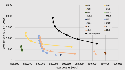
Fig. 3. Comparison of the five scenarios for laptop production.
4.2. Comparative Analysis of All Scenarios for Laptop Production
Figure 3 shows the results of the five scenarios obtained for laptop production. The yellow, green, blue, and red data markers represent the China, Malaysia, the United States, and Japan advanced scenarios, respectively. The figure legend indicates the RE utilization rate. For example, C0.1 indicates the China advanced scenario with an RE utilization rate of \(\alpha=0.1\).
The China, the United States, and Japan advanced scenarios exhibited poor cost-effectiveness compared with the Malaysia advanced scenario. The reasons underlying the poor cost-effectiveness in China, the United States, and Japan differed from one another. For the China advanced scenario, it was difficult to reduce the GHG emissions at a high RE utilization rate.
In this scenario, many Chinese suppliers with high GHG emissions should be selected to satisfy a high RE utilization rate. However, in the United States and Japan advanced scenarios, suppliers located in the United States or Japan with high procurement costs should be selected to satisfy the high RE utilization rate. Consequently, the Malaysia advanced scenario was the most cost-effective scenario, followed by the United States, China, Japan, and non-adoption scenarios, as shown in Fig. 3. The factors contributing to the cost-effectiveness of the Malaysia advanced scenario are summarized as follows.
-
・
Reduced transportation costs: Selecting Malaysian suppliers reduced the transportation distance to the assembly factory located in Malaysia, which minimized the transportation costs.
-
・
Competitive manufacturing costs: Among the four countries compared, Malaysia offered the lowest component manufacturing costs.
Given these factors, the frequent selection of Malaysian suppliers in the advanced scenario significantly reduced GHG emissions from electricity consumption while suppressing the increase in the total cost.
4.3. Analysis of Suppliers and Factories for Laptop Production
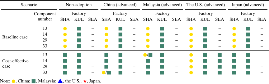
Table 4 summarizes the sourcing of key components for the baseline and cost-effective scenarios, as represented by the data markers in Fig. 2. The SHA, KUL, and SEA in Table 4 refer to Shanghai, Kuala Lumpur, and Seattle, respectively. Four key laptop components were associated with higher GHG emissions and procurement costs. For instance, for the baseline case of the non-adoption scenario, the board component (component #13) at the Shanghai factory was procured from a Chinese supplier, whereas for the cost-effective case, the board component was procured from Malaysian suppliers for both Shanghai and Kuala Lumpur factories. It shall be highlighted that the blue squares and red stars indicate the United States and Japanese suppliers, respectively; however, these suppliers were not selected for the cases in Table 4. The results indicated that at the Chinese factory, the suppliers for components #13 (board component), #14 (central processing unit), #29 (web camera + board), and #33 (wireless LAN card) switched to those in Malaysia to improve the cost-effectiveness in most cases. All these components, which were made of hybrid integrated circuits, were characterized by high GHG emissions and procurement costs. This finding indicated that switching to Malaysian suppliers for these components was key to reducing GHG emissions in a cost-effective manner.
In addition, the Seattle factory in the United States was opened only to attain cost-effectiveness in the United States advanced scenario. The United States factory procured all key components from Malaysian suppliers, even though RE100 suppliers were available in the United States without purchasing electricity. A Malaysian supplier was selected to reduce the procurement costs and GHG emissions. Moreover, Malaysian suppliers had a lower customs duty than Chinese suppliers because the rate of customs duty levied on products imported to the United States was lower for goods from Malaysia than for those sourced from China, with representative rates of 10% and 25%, respectively.
5. Analysis for Vacuum Cleaners
Similar to the laptop case, we implemented our proposed model to analyze the GHG emissions and total cost for the production of vacuum cleaners for five scenarios in four countries.
5.1. Trends of GHG Emissions and Total Cost for Vacuum Cleaner Production
The results for vacuum cleaners obtained using our proposed model are discussed in this section. The vacuum cleaner included components #12 (mesh filter) and #16 (upper filter) made from carbon fiber, which were characterized by high procurement costs and GHG emissions.
The total GHG emissions and total cost for each scenario are shown in Fig. 4. It is worth noting that the scales of the axes in each graph differ from one another.
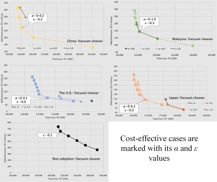
Fig. 4. Relationships between the GHG emissions and total cost for vacuum cleaner production.
The results showed that the GHG emissions could be reduced by 50% by changing the configuration of the supply chain, even without introducing the use of RE in the non-adoption scenario. However, these reductions were accompanied by a significant increase in the total cost. Compared with that for the baseline case (\(\varepsilon=0.0\)), the total cost was higher by a factor of \(\sim\)1.3 with a reduction in GHG emissions of 50%.
In the China advanced scenario, it was possible to achieve a maximum GHG reduction of \(\sim\)40% from the baseline value. However, this reduction increased the total cost drastically by USD 63,515.7. Thus, this scenario was not recommended because it was not cost-effective.
Furthermore, in this scenario, setting a high constraint on the RE utilization rate \(\alpha\) made reducing the GHG emissions difficult. In the baseline case, the GHG emissions from material production accounted for \(\sim\)96.5% of total GHG emissions. Switching suppliers from China to Malaysia, Japan, or the United States would be effective to reduce GHG emissions from material production. However, in this scenario, shifting production to locations outside China could reduce the RE utilization rate across the entire system. This made it impossible to obtain a solution that satisfied a certain level of RE utilization, as with laptops. Consequently, we did not observe any changes in the output results for an RE utilization rate of \(\alpha\geq 0.6\) with a GHG reduction rate of \(\varepsilon=0\).
The baseline GHG emissions in the Malaysia advanced scenario were the lowest compared with those in the other scenarios. The Malaysia advanced scenario was the only scenario in which the GHG emissions were less than 200 t-CO\(_2\)eq without constraints on the RE utilization rate \(\alpha\) and GHG reduction rate \(\varepsilon\). Similar to the China advanced scenario, setting a high RE utilization rate \(\alpha\) created a trade-off with GHG reduction. The GHG emissions from material production accounted for \(\sim\)94.8% of the total emissions in the baseline case, and shifting suppliers to the United States or Japan to reduce GHG emissions decreased the ratio of RE utilization, which made satisfying these constraints unfeasible. The most favorable results in terms of cost-effectiveness were obtained at \(\alpha=0\)–1.0 and \(\varepsilon=0.3\). The results confirmed that the constraint representing the RE utilization rate \(\alpha\) did not affect the results when the GHG reduction rate \(\varepsilon\) was set to \({\geq}30\)%. This was expected because the costs and GHG emissions at \(\varepsilon=0.4\) and 0.5 remained roughly the same regardless of the RE utilization rate \(\alpha\) as the supplier configuration was not changed. Specifically, for \(\alpha\geq 0.7\), the supplier configuration became constant regardless of the GHG reduction rate. The Chinese factory procured components from Chinese suppliers with high GHG emissions in the baseline case. Switching to Malaysian and Japanese suppliers that provided components with small GHG emissions enabled manufacturing to be carried out within the range of the installed 20-kW PV power generation capacity. Hence, it was possible to reduce GHG emissions by 40% (\(\varepsilon=0.4\)) even at high RE utilization rates such as \(\alpha=0.9\) or 1.0.
Three factories were opened in China, Malaysia, and the United States at \(\alpha=0\)–0.1 and \(\varepsilon=0.4\) in the United States advanced scenario. In this scenario, although the total cost increased due to the high cost of electricity in the United States, the GHG emissions were reduced by 70% relative to those of the baseline case. The supply chain configuration was changed from procuring most components from Chinese and Malaysian suppliers in the baseline case to sourcing components from the United States with lower GHG emissions. On the other hand, the total cost increased because of the high procurement costs of components from United States suppliers. When the RE utilization rate \(\alpha\) was 1.0, the total cost to reduce GHG emissions by 70% was USD 186,946, which was 13% higher than that for the baseline case. It shall be noted that for \(\alpha\geq 0.9\), we did not observe any changes in the supplier configuration regardless of the GHG reduction rate.
Similar to the United States advanced scenario, the GHG emissions could be reduced by 70% in the Japan advanced scenario, although the total cost increased due to the high cost of electricity in Japan. The total cost increased when this reduction was achieved by changing procurement sources from China and Malaysia to Japan or the United States. In this scenario, as well as in the United States advanced scenario, the supplier configuration remained constant for \(\alpha\geq 0.9\) regardless of the GHG reduction rate. In terms of cost-effectiveness, \(\alpha=0\)–0.1 and \(\varepsilon=0.5\) were considered to be highly cost-effective.
5.2. Comparative Analysis of All Scenarios for Vacuum Cleaner Production
Figure 5 shows the results of the five scenarios for vacuum cleaner production. The solutions located in the lower-left region of the graph were considered more cost-effective. In the United States and Japan advanced scenarios, the cost-effectiveness was lower due to a significant increase in cost despite the higher reduction in GHG emissions. Conversely, in the China advanced scenario, although the increase in the total cost was suppressed at lower GHG reduction rates, the results for this scenario indicated poor cost-effectiveness. The minimum GHG emissions in the China advanced scenario were 172 t-CO\(_2\)eq, which were higher than the minimum emissions of other advanced scenarios by \(\sim\)95 t-CO\(_2\)eq.
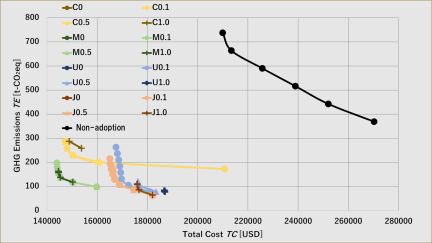
Fig. 5. Comparison of the five scenarios for vacuum cleaner production.
Therefore, the cost-effectiveness of the scenarios was ranked in the following order: Malaysia \(>\) Japan \(>\) the United States \(>\) China \(>\) non-adoption scenario. It is evident from the results that the Malaysia advanced scenario was the most cost-effective option. The factors contributing to the optimality of the Malaysia advanced scenario are summarized as follows:
-
・
Reduction in transportation costs: Selecting Malaysian suppliers reduced the transportation distance to the assembly factory located in Malaysia, thereby minimizing the transportation costs.
-
・
Competitive manufacturing costs: Among the four countries compared, Malaysia offered the lowest component manufacturing costs.
The frequent selection of Malaysian suppliers in the Malaysia advanced scenario significantly reduced GHG emissions from electricity consumption while suppressing the increase in the total cost due to these factors. Consequently, the Malaysia advanced scenario was the most cost-effective option for reducing GHG emissions.
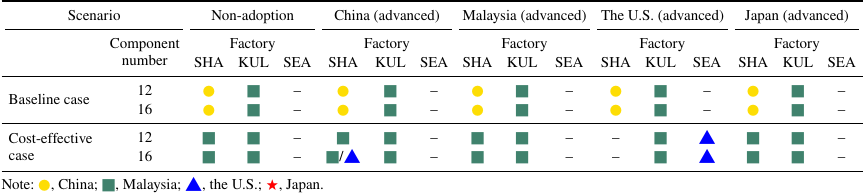
5.3. Analysis of Suppliers and Factories for Vacuum Cleaner Production
Table 5 summarizes the sourcing of key components for the baseline case and the case in which cost-effectiveness was considered for each scenario. The results indicated that at the Chinese factory, the suppliers for components #12 (mesh filter) and #16 (upper filter) consistently changed from suppliers in China to those located in Malaysia or the United States when cost-effectiveness was prioritized. Both of these components used carbon fiber as the raw material and were characterized by high GHG emissions and procurement costs.
The results demonstrated that switching suppliers for components with high GHG emissions from China to Malaysia could reduce GHG emissions without incurring significant costs, even for a factory located in China. Compared with laptops, the three factories were not opened in the United States advanced scenario, as shown in Tables 4 and 5. In the United States advanced scenario, which was the cost-effective scenario for vacuum cleaner production, factories were only opened in Malaysia and the United States. The Seattle factory in the United States procured components #12 (mesh filter) and #16 (upper filter) from domestic suppliers.
5.4. Comparison of the Results Between Laptops and Vacuum Cleaners
Both laptops and vacuum cleaners shared notable trends. For example, the Malaysia advanced scenario was the most cost-effective scenario among the five scenarios for both products. One key difference was the higher total cost of the laptop at higher RE utilization rates \(\alpha\) in the United States and Japan advanced scenarios. This discrepancy was likely because Malaysian suppliers continued to be selected for the production of vacuum cleaners to a certain extent even as \(\alpha\) increased, whereas they were selected less frequently for laptop production. In addition, the manufacturing of laptop components was characterized by higher power consumption compared with the manufacturing of vacuum cleaner components. Consequently, the RE generation capacity of 20 kW allocated to each supplier was insufficient to meet the power demand. Thus, a high RE utilization rate \(\alpha\) was required to procure components from RE100 suppliers. The higher RE utilization rates in the United States and Japan advanced scenarios led to many components being procured from these countries. For vacuum cleaners, selecting suppliers in the United States or Japan was possible even at a high RE utilization rate \(\alpha\) or GHG emission reduction rate \(\varepsilon\), unlike that for laptops. Consequently, the potential for reducing GHG emissions was lower for laptop production compared with that for vacuum cleaner production, and setting a high GHG reduction rate \(\varepsilon\) was not feasible.
Based on the results described in Sections 4.3 and 5.3, when prioritizing cost-effectiveness, changes in suppliers tended to focus on components with high GHG emissions. Specifically, suppliers of components with high GHG emissions and procurement costs shifted from China to Malaysia.
Furthermore, two factories were opened in most cases. In several cases, a factory could be opened in the United States instead of in China. Even in cases without changes in factory location, suppliers of components with high GHG emissions and procurement costs were switched from Malaysia to the United States or Japan.
6. Conclusion
In this study we developed an RE-based GSCN model where we considered GHG emissions from electricity consumption during component production and GHG emissions from material production to attain both the target RE utilization and GHG reduction rates. The GHG emissions from electricity consumption were dependent on the available and used amounts of RE. Our model enabled suppliers to purchase electricity generated by external non-RE sources when the RE systems alone could not satisfy the power demand. Furthermore, the suppliers could not supply the components when they could not meet the required RE utilization rate in keeping pace with their productivity.
We compared the results between the production of laptops and vacuum cleaners, and we found that the advanced scenarios could reduce GHG emissions at a lower total cost than the baseline case for both laptops and vacuum cleaners. In particular, the Malaysia advanced scenario showed high cost-effectiveness, owing to its low procurement costs and low GHG emissions from material production. However, as laptops consumed substantially more electricity during component manufacturing than vacuum cleaners, the 20-kW RE generation capacity for the other three countries could be a critical constraint. Consequently, for laptops, achieving a high RE utilization rate forced the selection of suppliers with higher costs. Based on these findings, when prioritizing cost-effectiveness, Malaysian suppliers should introduce RE facilities to provide components for factories in Malaysia, China, or the United States.
However, our proposed model has a few limitations, which are listed as follows:
-
・
Although we incorporated a predetermined amount of RE, we did not address the installation cost of RE facilities.
-
・
We did not consider carbon policies such as carbon tax and carbon cap-and-trade, although many countries have implemented these carbon policies to reduce GHG emissions in the GSCN.
-
・
We assumed that the suppliers in each country could provide components of the same quality. We assumed that only the procurement costs and GHG emissions differed among suppliers in formulating the model.
-
・
The RE utilization and GHG reduction rates were set as hard constraints. Decision-makers often set these targets at ideal levels. Hence, the RE utilization and GHG reduction rates will be useful for decision-makers to obtain a solution that does not achieve the set ideal target but is close to the target.
Future research should consider the allocation of funds to suppliers in transitioning to clean energy, which will motivate them to adopt green energy policies and practices and extend the applicability of our proposed model. For example, Apple Inc. provides a green program to support suppliers’ RE100 achievement by investing in suppliers to transition to clean energy 10. Moreover, studies should be carried out to extend our model to consider a reverse supply chain that encompasses the collection and recycling processes of used products 26. Furthermore, various carbon policies such as carbon taxes and cap-and-trade systems should be incorporated to evaluate their effects on the design of the supply chain network. Future work should also consider economic fluctuations, including tariffs and variations in electricity costs, and evaluate the differences in architectural products 27.
Acknowledgments
This work was supported by JSPS KAKENHI Grant-in-Aid for Early-Career Scientists (grant number: JP26K17605) and Scientific Research (B) (grant number: JP23K26329). During the preparation of this work, the authors used “Gemini 3.5 Thinking” to refine the language in order to improve the clarity and readability of the text. After using this tool, the authors reviewed and revised the content as required. The authors take full responsibility for the contents of the published article.
- [1] Ministry of the Environment, “Annual report on the environment, in Japan 2025.” https://www.env.go.jp/policy/hakusyo/r07/eng/2025_all.pdf [Accessed August 25, 2026]
- [2] M. J. Meixell and V. B. Gargeya, “Global supply chain design: A literature review and critique,” Transp. Res. E: Logist. Transp. Rev., Vol.41, No.6, pp. 531-550, 2005. https://doi.org/10.1016/j.tre.2005.06.003
- [3] D. J. Zhang, S. S. Dabadghao, and M. Udenio, “Global sourcing under tariffs: A perspective of time series analysis,” Int. J. Prod. Econ., Vol.280, Article No.109473, 2025. https://doi.org/10.1016/j.ijpe.2024.109473
- [4] Sharp Corporation, “2025 sustainability report,” 2025. https://global.sharp/corporate/eco/report/pdf/ssr2025_e.pdf?v=2025 [Accessed August 25, 2026]
- [5] J. W. Lee et al., “Optimal sourcing strategy for enterprises to achieve 100% renewable energy,” Energy Rep., Vol.8, pp. 14865-14874, 2022. https://doi.org/10.1016/j.egyr.2022.10.443
- [6] Microsoft Corporation, “2025 Environmental Sustainability Report: Accelerating progress to 2030,” 2025. https://cdn-dynmedia-1.microsoft.com/is/content/microsoftcorp/microsoft/msc/documents/presentations/CSR/2025-Microsoft-Environmental-Sustainability-Report.pdf [Accessed August 25, 2026]
- [7] Panasonic Corporation, “Sustainability data book 2025,” 2025. https://holdings.panasonic/global/corporate/sustainability/pdf/sdb2025e.pdf [Accessed August 25, 2026]
- [8] Seiko Epson Corporation, “Epson group sustainability report 2025,” https://corporate.epson/en/sustainability/report/pdf/2025/epson_sr2025_all_e.pdf [Accessed August 25, 2026]
- [9] L. Präger, J. Woytowicz, R. Reitberger, and W. Lang, “LCA-based calculation of GHG Protocol Scope 3: A bottom-up approach to determine GHG emissions of the construction activity of municipalities,” Build. Environ., Vol.285, Part A, Article No.113502, 2025. https://doi.org/10.1016/j.buildenv.2025.113502
- [10] Apple Inc., “Annual green bond impact report: Fiscal year 2023 update,” 2024. https://s2.q4cdn.com/470004039/files/doc_downloads/additional_reports/2023/apple_greenbond_report_fy2023.pdf [Accessed August 25, 2026]
- [11] Y. Nagai, “Planning method of a global supply chain network considering RE100 contract of photovoltaic power generation,” Bachelor’s Thesis, The University of Electro-Communications, 2025 (in Japanese).
- [12] M. Kotegawa, Y. Kinoshita, and T. Yamada, “Global supply chain network design under cap-and-trade system and analysis of carbon price and emission allowance,” Green Low-Carbon Econ., Vol.3, No.2, pp. 159-170, 2025. https://doi.org/10.47852/bonviewGLCE42022351
- [13] International Energy Agency, “Renewables 2025: Analysis and forecasts to 2030,” 2025. https://iea.blob.core.windows.net/assets/76ad6eac-2aa6-4c55-9a55-b8dc0dba9f9e/Renewables2025.pdf [Accessed August 25, 2026]
- [14] H.-W. Lo, C.-J. Pai, and M. Deveci, “A multi-objective model for integrated supplier order allocation and supply chain network transportation planning decision-making,” Inf. Sci., Vol.689, Article No.121487, 2025. https://doi.org/10.1016/j.ins.2024.121487
- [15] R. Eslamipoor and A. Sepehriyar, “Promoting green supply chain under carbon tax, carbon cap and carbon trading policies,” Business Strategy and the Environment, Vol.33, No.5, pp. 4901-4912, 2024. https://doi.org/10.1002/bse.3721
- [16] T. Nagao, H. Ijuin, Y. Kinoshita, K. Nagasawa, and T. Yamada, “Designing global supply chain network under carbon border adjustment mechanism for low-carbon economy,” Int, J. Adv. Manuf. Technol., Vol.146, No.3, pp. 1567-1583, 2026. https://doi.org/10.1007/s00170-025-17186-z
- [17] M. A. Edalatpour, A. M. Fathollahi-Fard, S. M. J. M. Al-e-Hashem, and K. Y. Wong, “Global sustainable closed-loop supply chain network considering incoterms rules and advertisement impacts,” J. Ind. Inf. Integr., Vol.42, Article No.100737, 2024. https://doi.org/10.1016/j.jii.2024.100737
- [18] Y. Yoshizaki, T. Yamada, N. Itsubo, and M. Inoue, “Material based low-carbon and economic supplier selection with estimation of GHG emissions and affordable cost increment for parts production among multiple Asian countries,” J. Jpn. Ind. Manag. Assoc., Vol.66, No.4E, pp. 435-442, 2016. https://doi.org/10.11221/jima.66.435
- [19] K. Horiguchi, M. Tsujimoto, H. Yamaguchi, and N. Itsubo, “Development of greenhouse gases emission intensity in eastern Asia using Asian international input-output table,” Proc. 7th Meet. Inst. Life Cycle Assess. Jpn., pp. 236-239, 2012 (in Japanese). https://doi.org/10.11539/ilcaj.2011.0.116.0
- [20] T. Suzuki et al., “Study of assembly reliability evaluation,” Proc. 13th Des. Syst. Conf., pp. 262-265, 2003 (in Japanese). https://doi.org/10.1299/jsmedsd.2003.13.262
- [21] Y. Ueno et al., “Study of assembly reliability evaluation method: Application to piping work of heavy equipments,” Proc. 14th Des. Syst. Conf., pp. 168-171, 2004 (in Japanese). https://doi.org/10.1299/jsmedsd.2004.14.168
- [22] Ministry of Internal Affairs and Communications, “New international comparisons of GDP and consumption based on purchasing power parities for the year 2014 gross domestic product at current PPPs and current exchanges rates” (in Japanese). https://www.soumu.go.jp/toukei_toukatsu/index/kokusai/icp.html [Accessed August 25, 2026]
- [23] Ministry of Economy, Trade and Industry, “Census of manufacture” (in Japanese). http://www.meti.go.jp/statistics/tyo/kougyo/result-2/h17/kakuho/hinmoku/index.html [Accessed August 25, 2026]
- [24] H. Takatori, “Technical progress of large size injection molding machine,” Seikei-Kakou (J. Jpn. Soc. Polym. Process.), Vol.18, No.10, pp. 729-734, 2006 (in Japanese). https://doi.org/10.4325/seikeikakou.18.729
- [25] NTT DATA Mathematical Systems Inc., “Nuorium Optimizer.” https://www.msi.co.jp/english/nuopt.html [Accessed August 25, 2026]
- [26] J. Koketsu, A. Ishigaki, H. Ijuin, and T. Yamada, “Variability specific to a closed-loop supply chain with product deterioration,” Int. J. Automation Technol., Vol.16, No.6, pp. 727-736, 2022. https://doi.org/10.20965/ijat.2022.p0727
- [27] S. Yamada, Y. Komatsu, S. Bracke, and M. Inoue, “Product architecture derivation methodology based on multi-objective design structure matrix integration and supply chain evaluation,” Int. J. Automation Technol., Vol.19, No.2, pp. 88-99, 2025. https://doi.org/10.20965/ijat.2025.p0088
Appendix
Appendix A. All Reduction and Renewable Energy Utilization Rates for Laptops and Vacuum Cleaners
Figures 6 and 7 show the results of all reduction and renewable energy utilization rates for laptops, whereas Figs. 8 and 9 show those for vacuum cleaners.
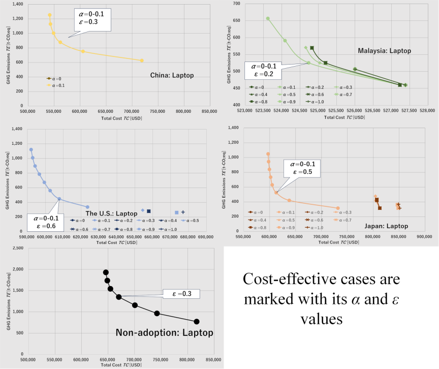
Fig. 6. Relationships between the GHG emissions and total cost for laptop production. The results for all RE utilization rates are presented here.
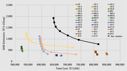
Fig. 7. Comparison of the five scenarios for laptop production. The results are presented for all RE utilization rates.
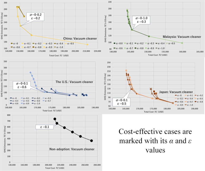
Fig. 8. Relationships between the GHG emissions and total cost for vacuum cleaner production. The results for all RE utilization rates are presented here.
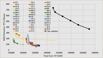
Fig. 9. Comparison of the five scenarios for vacuum cleaner production. The results are presented for all RE utilization rates.
This article is published under a Creative Commons Attribution-NoDerivatives 4.0 Internationa License.