
Research Paper:
Simulating Feedback System for Calibrating Parameters of Circular Consumer Incentive Models
Raul Carlsson*,†
 and Tatiana Nevzorova**
*Carlson’s FactSky
Ansgariigatan 17, , Sweden
†Corresponding author
**Business design, RISE Research Institutes of Sweden
Stockholm, Sweden

The main methodological contribution is treating consumer behaviour as an endogenous, probabilistic system component whose response to information and incentives can be parameterised and tested rather than assumed as fixed. Behavioural responses are modelled as functions of incentive type, communication frequency, timing, and decay over time. This enables systematic testing of strategies such as point-of-sale information, brand communication, recurring engagement (e.g., recurring customer reminders), second-hand market promotion, and varying levels of monetary incentives. These behavioural parameters are linked to material flows within a modular circular value chain, allowing analysis of how individual decisions scale to system-level environmental and economic outcomes. Applied to a denim case study, the model shows how changes in consumer response probabilities alter the distribution between virgin production, reuse, repair, remanufacturing, and recycling. In the illustrative denim experiment, progressively stronger intervention conditions reduce modelled virgin-material demand, 100-year global warming potential (GWP100) and cost. Overall, the findings show that circular business model performance can be sensitive to consumer participation, while the magnitude of the effect remains conditional on the behavioural and technical assumptions. The tool enables pre-implementation testing of incentive strategies, offering a novel decision-support approach for companies and policymakers seeking to align consumer behaviour with circular economy innovations. The same structure identifies which consumer-response and decay parameters require empirical calibration.
Incentivizes agents to act circular
1. Introduction
The transition from a linear to a circular economy (CE) aims to retain the value of products, components, and materials through reuse, repair, refurbishment, remanufacturing, and recycling. Yet, technical aspects, such as product design, reverse logistics, and circular business models (CBMs) do not ensure that products enter these loops; the outcomes depend on consumer participation decisions when acquiring, using, maintaining, returning, reselling, repairing, or discarding products 1,2,3,4,5,6.
Consumer behaviour directly shapes product lifetime, collection, return flows, demand for second-hand or remanufactured products, and virgin-production substitution. Still, favourable attitudes often fail to produce repair, reuse, return, or otherwise adopt circular offers 2,3,4,5,6 because of limited awareness, inconvenience, risk, price, product condition, distrust, or due to unavailable services. CBM performance may therefore fall well below any of its technical potentials.
Information and incentives may narrow this gap, but effects depend on type, timing, repetition, channel, and context, and the significance of information and facts also decays over time. Point-of-sale information can shape purchases; reminders can prompt maintenance, repair, or returns; social signals can influence norms; and monetary rewards can shift return, resale, or disposal choices. Because real-world testing is costly and behavioural changes can propagate through logistics, markets, production, and environmental impacts, pre-implementation modelling can cut costs and can also serve as market validators and verifiers as models may be calibrated with real cases.
Environmental assessments often represent consumer actions through fixed assumptions or limited sensitivity scenarios 7. Although behavioural simulations can capture heterogeneous decisions and emergent outcomes in CBMs, product life cycles, and resource recovery 8,9,10,11,12, configurable incentives, time-dependent response probabilities, and process-based material flows are rarely integrated for decision support. Practitioners therefore lack a transparent way to determine how strong, persistent and frequent a message must be to significantly improve the real system performance.
This study develops a modular simulation linking life-cycle inventory flows to probabilistic consumer decisions at use and post-use nodes. These coordinated activities are treated as a post-manufacturing production system. Scenario parameters cover message and incentive type, communication timing and frequency, and influence decay; response probabilities redirect flows among continued use, repair, second-hand use, remanufacturing, recycling, and to final incineration and landfill.
Unlike conventional life cycle assessment (LCA), the simulation targets behavioural leverage points, although it has not yet been calibrated with real-world customer communication campaign data. The denim case models reuse, repair, and component recovery environmentally and economically, initially using 100-year global warming potential (\(\mathrm{GWP}_{100}\)), with scope to add indicators for other product contexts.
The study asks: (1) how can incentivised consumer decisions be represented as configurable parameters in a circular life-cycle simulation, and (2) how do parameter changes affect material flows and environmental outcomes? It contributes a feedback-oriented structure linking interventions, behavioural responses, circular flows, and life-cycle indicators; demonstrates it with denim; and identifies calibration data needs. Following ISO 14040/14044 and ISO 59020 13,14,15, the framework embeds message timing, format, and repetition within system modelling rather than duplicating conventional LCA.
The study was developed with Swedish industry partners and resulted in a simulation tool for designing communication, policy, and market-based incentives for circular practices. It contributes by integrating LCA with parameterised consumer decisions, treating information, engagement, and monetary incentives as controllable variables, and showing how response probabilities propagate through circular value chains to affect material flows and environmental outcomes. Incentive design thus becomes a model input and consumer response a quantifiable, probabilistic component of CE performance.
Section 2 reviews prior work and the methodological gap; Section 3 presents the simulation method; Section 4 defines the denim case; Section 5 reports results; Section 6 discusses implications, limitations, and calibration; and Section 7 concludes.
2. Literature Review
Review scope and selection. Sources were identified by citation chaining from established and recent reviews, supplemented by targeted searches combining terms related to CE or CBMs with consumer behaviour, incentives, repair, reuse, return, simulation, agent-based modelling (ABM), and LCA. English-language peer-reviewed studies were retained when they informed at least one of four links in the proposed causal chain: (1) consumer decisions that enable circular strategies, (2) determinants or incentives affecting those decisions, (3) formal representation of behaviour, or (4) propagation of behavioural outcomes into product, material, economic, or environmental performance. Design, business-model, logistics, and policy studies were included only where they clarified one of these links 16,17,18,19,20,1,21,22,2,3,4,5,6,7,8,9,10,11,12,23,24. The review is intended to establish the conceptual and methodological positioning of the model rather than to claim an exhaustive systematic review.
Consumer behaviour in circular systems. CE consumption involves more than purchasing products with environmental attributes; it includes acceptance of access-based and product-service offers, maintenance, repair, prolonged use, sharing, resale, return, sorting, and recycling 1,4. These actions determine whether technically available loops are realised. Product design and user support can strengthen perceived ability to diagnose faults and repair products 18,2, while empirical studies show that acquisition, use, repair, and end-of-life practices vary across users and contexts 3. Consumer acceptance of CBMs is influenced by convenience, price, perceived quality and risk, ownership preferences, trust, and the value proposition offered by the provider 5,6,24. Thus, a CBM’s environmental potential cannot be inferred from technical loop design alone.
Incentives and behavioural determinants. The literature distinguishes informational interventions, economic incentives, social influence, and enabling conditions. Information can increase awareness and perceived competence, but information alone may be insufficient when repair services, collection systems, or attractive circular alternatives are unavailable 18,2,3,4,5,6. Monetary incentives can alter the comparative utility of return, reuse, or circular acquisition, whereas communication by brands, peers, or institutions may affect trust and social norms. Digital traceability and product information infrastructures can support decisions by making product condition, repair options, and environmental attributes visible 19,25,26. However, responses are heterogeneous and context dependent, and the effect of a message may weaken between exposure and the relevant decision. These findings support representing incentive effects as variable probabilities rather than assuming uniform compliance. These two features, heterogeneous response and decay between exposure and decision, are represented explicitly in the behavioural and time-dependent state functions introduced in Sections 3.2 and 3.3.
Behaviour in LCA and sustainability assessment. Conventional LCA provides a process-based account of environmental impacts across a product system 13,14, but consumer behaviour is often represented through average values, fixed allocation factors, or discrete scenarios. Corona et al. 7 found that circular-packaging LCAs commonly rely on behavioural assumptions and mainly address variability through scenario and sensitivity analysis. This can test alternative outcomes, but it does not explain how an intervention changes behaviour or capture interactions among decisions over time. Coupling behavioural models with LCA can instead generate foreground inventory flows—the process and flow data directly modelled for the studied product system—from simulated choices and support dynamic, spatial, or consequential assessment 11,12.
Simulation approaches. System dynamics is useful for aggregate feedback and stock-flow relationships, while discrete-event simulation represents process sequences and operational constraints. Game-theoretic models examine strategic responses among firms, consumers, and policymakers 22. ABM represents individual or organisational actors with decision rules and can capture heterogeneity, bounded rationality, social influence, diffusion, and emergent system behaviour. Lieder et al. 8 used ABM to study consumer acceptance of circular business-model changes, and Koide et al. 10 modelled product acquisition, repair, obsolescence, and discharge to assess multiple circular strategies. Reviews of CE-oriented ABM show growing applications in consumer behaviour, industrial symbiosis, waste management, logistics, and sharing systems, while also noting high parameter requirements and difficult empirical validation 9,23.
Integration of behavioural simulation and environmental flows. ABM-LCA coupling has been proposed to improve modelling of behaviour-driven use phases and evolving foreground systems 11,12. In CE applications, simulation can reveal thresholds, bottlenecks, rebound effects—where gains are partly offset by induced changes in demand or use—and nonlinear consequences that fixed scenarios may conceal. For example, increased acceptance of a refurbished offer may be constrained by the number and condition of returned products, and additional collection or transport may offset part of the environmental benefit 10. These studies establish the value of behavioural simulation, but they also show that model usefulness depends on a clear mapping from interventions and evidence to behavioural parameters and from individual choices to physical flows.
Research gap and positioning. Prior studies provide important accounts of circular consumption, consumer acceptance, behavioural determinants, and ABM-based diffusion. However, three elements are rarely combined in a single, practitioner-oriented tool: configurable representations of specific incentive interventions, time-dependent response functions that include repeated communication and decay, and direct propagation of the resulting decisions through a modular life cycle inventory of circular pathways. The present study addresses this narrower gap. It does not claim to replace empirically grounded ABM or behavioural experiments. Instead, it provides an exploratory feedback system for testing incentive configurations, identifying behavioural response thresholds, and determining which parameters require empirical calibration before implementation.
The reviewed literature therefore supports the modelling chain used in this study: incentive design influences response probabilities; response probabilities allocate products among use and post-use decisions; these allocations change circular material flows; and the altered flows affect resource use, environmental performance and cost. This study addresses this gap by integrating behavioural response functions directly into a life cycle-based simulation environment. Section 3 translates this chain into the generic simulation framework.
3. Methodology
The methodology operationalises the intervention-to-flow chain established in Section 2 and is specified independently of the denim application. Reported outputs are generated only after these layers have been executed. This separation is important because it distinguishes the generic model equations from the case-specific intervention settings introduced in Section 4.
3.1. Integrated Behavioural/Circular-System Architecture
Figure 1 gives the computational architecture. Scenario controls do not directly prescribe environmental or economic outcomes. They first alter the information and economic inputs received by individual agents. The agent layer converts those inputs into probabilities for the modelled decisions. The annual state update then carries the retained information state and use-related consequences into the next model year. Aggregated behavioural outputs are supplied to the circular-system interfaces, which in turn determine the material flows entering the life-cycle impact and cost(1) calculations (see Appendix A).
The architecture carries state over time rather than treating each model year as an independent scenario. Information can persist and decay between years, and garment-specific communication is linked to expected washing events. A change in the probability of sparse washing, meaning washing less frequently than the baseline frequency, therefore changes expected washing frequency, which changes the number of garment-information exposures entering the next annual update. Repair and washing outcomes also enter the effective-lifetime calculation. The resulting feedback is shown explicitly in Fig. 1.
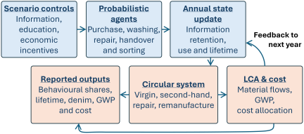
Fig. 1. Integrated behavioural/circular-system simulation architecture. Scenario controls act on agent-specific decision functions; the annual state update carries retained information and use-related state to the next model year; aggregated behavioural outputs are passed to the circular system and to LCA and cost calculations. The upper blue boxes represent intervention, behavioural, and time-dependent state functions; the lower neutral boxes represent physical-system calculation and reported-output functions.
3.2. Behavioural Decision Functions and Consumer Heterogeneity
Model parameters and probability and distribution formulas. Let \(i\) denote an agent, \(t\) the model year, \(a\) a binary action, and \(k\) a purchase alternative. Each agent has a fixed information-receptivity multiplier \(r_i^{\mathrm{I}}\) and economic-receptivity multiplier \(r_i^{\mathrm{E}}\). Let \(I_{i,t}\) denote the retained general-information stock, \(I_{i,t}^{\mathrm{P}}\) the information available at the purchase decision, and \(E_s\) the economic-incentive intensity in scenario \(s\). For the four binary actions, sparse washing, repair, handover to second hand, and correct sorting/recycling, the executable model uses the complementary-exponential response function
Equation (1) can be read from the complementary probability. At baseline, let \({B=1-p_{a}^{0}}\) be the probability of not taking action \(a\). The model assumes that information and economic inputs reduce this remaining non-action probability to \({B' = B{f(i,e)}}\), where \({0 < f(i,e) \leq 1}\). Therefore, \({p = {1-B'} = {1- (1-p_{a}^{0})f(i,e)}}\). In the implemented model, \({f(i,e) = e^{-\beta_{a}r_{i}^{\mathrm{I}} I_{i,t} - \gamma_{a}r_{i}^{\mathrm{E}}E_{s}}}\), so the information and economic terms act as separate multiplicative reduction factors on the remaining non-action probability. This is an implemented simulation response function rather than an empirically estimated behavioural law. With zero information and zero economic input, Eq. (1) returns the stated baseline probability. Positive input changes the probability monotonically while keeping it within \({[0, 1]}\), so no separate rule is required to force probabilities back into this range. Temporal persistence is represented separately through the information-state dynamics in Eqs. (4)–(6). The literature reviewed in Section 2 motivates the choice of decision nodes and intervention types; the numerical response coefficients are explicit model assumptions and are therefore examined by sensitivity analysis rather than presented as empirically measured response effects.
Consumer purchase decisions are represented by four mutually exclusive pathway alternatives in the implemented model: virgin/new, second-hand, repaired/refurbished, and remanufactured product supply. Section 4 instantiates these alternatives for the denim case. The model first calculates a positive weight for each alternative,
Equation (3) then divides each adjusted weight by the sum of all four weights, so that the decision probabilities sum to one for every agent and year and reproduce the baseline mix when all information and economic inputs are zero. Point-of-purchase information enters \(I_{i,t}^{\mathrm{P}}\) and can therefore alter the relative purchase weights without being added to the retained general-information stock. The case-specific values of the baseline probabilities/shares and response coefficients are declared in Section 4.1 rather than in the generic method.
Consumer heterogeneity is represented explicitly rather than by one representative consumer. Each agent carries fixed information- and economic-receptivity multipliers \(r_i^{\mathrm{I}}\) and \(r_i^{\mathrm{E}}\), and the same agent-specific multipliers are preserved through the temporal updates. The executable model supports two aggregation modes. In expected-population mode, Eqs. (1)–(3) are evaluated for every agent and the resulting probabilities are averaged; in realised-action mode, actions are sampled from those same probabilities. The population size, receptivity range, pseudorandom-number seed and aggregation mode used in the denim experiment are specified in Section 4.
3.3. Time-Dependent Information State and Feedback
Information is represented as a stock that can be reinforced by recurring communication and reduced by memory decay. The information half-life \(h\) is the time over which the retained information stock is assumed to fall by half in the absence of reinforcement. For an information half-life \(h\), the annual retention factor is
The half-life and intervention doses are scenario controls whose numerical values are specified for the denim experiment in Section 4; here, dose means the dimensionless information input added by an intervention, not a physical quantity. Let \(d_s^{\mathrm{M}}\) be the annual membership dose, \(d_s^{\mathrm{G}}\) the garment-information dose per wash, \(d_s^{\mathrm{T}}\) and \(d_s^{\mathrm{Pr}}\) the one-time theoretical and practical education doses, and \(d_s^{\mathrm{POS}}\) the point-of-purchase dose. The retained general-information stock is initialised as
The point-of-purchase dose is available at the purchase decision in each model year but is not retained in the general-information stock. This separation allows purchase-specific information to change purchase weights without necessarily changing the retained information driving use-phase binary actions. The sparse-washing probability is translated into expected washing frequency by the implemented linear mapping
3.4. Integration with Circular Material Flows, LCA, and Cost
The behavioural layer supplies a set of aggregated outputs to the existing circular-system calculation rather than replacing the life-cycle model. This set contains the normalised purchase shares, sparse-washing share, repair-action share, handover share, correct-sorting/recycling share, expected washing frequency, and effective lifetime. These quantities determine the corresponding product and material pathways. The downstream calculation then resolves market quantities, required material, looped and virgin material contributions, post-use routing, \(\mathrm{GWP}_{100}\) and allocated cost using the case-specific technical coefficients.
An information or economic intervention never changes \(\mathrm{GWP}_{100}\) or cost directly. It changes agent-level information and economic inputs; these change decision probabilities; the aggregated decisions change use, lifetime and circular-flow routing; and only then do the physical, environmental and economic calculations change. The resulting outputs are therefore conditional consequences of the stated behavioural and technical assumptions.
3.5. Execution, Aggregation, and Reproducibility
The authoritative executable implementation is not provided but run input and output data are supplied as Additional Material S1.(2) Run controls expose the agent population, simulation horizon, information half-life, scenario information inputs, response parameters, aggregation mode, and pseudorandom-number seed without changing the response equations. Expected-population aggregation and realised-action sampling therefore execute the same agent probabilities through different aggregation branches. The exact settings used for the denim experiment are specified in Section 4; parameter locations, run identifiers, balance checks and machine-readable outputs are provided in Additional Material S1.
4. Denim Case and Experimental Setup
The generic method was instantiated as an illustrative denim experiment. The case is designed to test whether the implemented behavioural/circular-system architecture can propagate specified information, education, and economic conditions through consumer decisions to physical, environmental and cost outputs. It is not an empirically calibrated consumer study. The intervention doses, behavioural response coefficients and fixed technical coefficients are model inputs; purchase shares, use behaviours, effective lifetime, material flows, \(\mathrm{GWP}_{100}\), and costs are calculated outputs. No primary consumer-response dataset was collected or used to estimate the response coefficients in this study. Consumer survey data therefore do not enter the parameterisation; the specified values are entered directly as controlled model and scenario assumptions. The numerical results therefore quantify conditional consequences of the stated assumptions and should not be interpreted as forecasts of observed consumer behaviour.
4.1. Case Boundary and Baseline Assumptions
The case maintains a market of 1,000,000 pairs of jeans and follows the same population through model years Y0–Y5, where Y0 denotes the initial simulation year and Y1–Y5 the five subsequent annual updates. The main simulation population contains \(N=\textrm{5,000}\) agents generated using pseudorandom-number seed 1729. Each agent has fixed information- and economic-receptivity multipliers centred close to one and spanning approximately 0.5–1.5 in the generated population; the same agent-specific multipliers are retained across years. Main-scenario and sensitivity runs use expected-population aggregation, while realised-action sampling is reserved for the implementation reproducibility check described in Section 4.3.
At zero intervention, the specified purchase baseline is 89% virgin, 5% second hand, 5% repaired/refurbished, and 1% remanufactured. Baseline probabilities for sparse washing, repair, handover to second hand, and correct sorting/recycling are 0, 0.03, 0.80, and 0.58, respectively. The information half-life is \(h=2\) years. The base washing frequency is \(W_{0}=2\) washes/year with \(\delta_{\mathrm{W}}=0.5\); the base lifetime is \(L_{0}=5\) years, a repaired pair receives \(\Delta L_{\mathrm{repair}}=2\) additional years, and \(\lambda_{\mathrm{W}}=1/12\) year per avoided annual wash. Table 1 reports the corresponding behavioural baselines and response coefficients used in Eqs. (1)–(3).
These baseline values and physical-link coefficients are pre-specified experimental assumptions. Information inputs are expressed in an internal, dimensionless information unit (IU); economic-incentive input is expressed on a separate internal, dimensionless scenario scale. They were selected to provide a non-trivial baseline from which several circular pathways can increase while preserving a dominant virgin-purchase share. They are not claimed to represent a national denim market or a measured consumer population. This distinction is important because the purpose of the experiment is to demonstrate and stress-test the model’s propagation logic; empirical calibration and external validation remain future work.
| Decision class / component order | Baseline \(p^0\) / \(s^0\) | \(\beta\) per IU | \(\gamma\) per economic-incentive unit | Information state |
| Binary actions (sparse; repair; handover; sorting) | 0.00; 0.03; 0.80; 0.58 | 0.20; 0.20; 0.10; 0.12 | 0.20; 0.50; 0.30; 0.30 | General \(I\) |
| Purchase alternatives (virgin; second-hand; repaired/refurb.; reman.) | 0.89; 0.05; 0.05; 0.01 | 0.00; 0.30; 0.30; 0.35 | 0.00; 0.50; 0.50; 0.50 | Purchase \(I^\mathrm{P}\) |
Note: Within each row, parameter values follow the component order shown in the first column. \(\beta\) and \(\gamma\) are specified case-response coefficients per corresponding information or economic-incentive input unit. None of these coefficients was estimated from primary consumer-response data in this study.
4.2. Intervention Ladder and Exact Scenario Implementation
Six nested intervention scenarios, labelled S0–S5, define a progressive ladder from no intervention to the combined information, education and economic case. S0 is the no-intervention baseline; S1–S5 successively add the intervention components shown in Table 2. Information intensity is expressed in IU, and the economic incentive on the internal economic-incentive scale defined above. These scales are computational inputs, not survey scores or monetary amounts. Table 2 gives the complete scenario matrix.
| Scenario | Intervention description | Point-of-purchase IU | Membership IU | Garment IU | Theory IU | Practical IU | Economic intensity |
| S0 | Baseline – no intervention | 0 | 0 | 0 | 0 | 0 | 0 |
| S1 | Point of purchase only | 1 | 0 | 0 | 0 | 0 | 0 |
| S2 | S1 + annual membership | 1 | 0.2/year | 0 | 0 | 0 | 0 |
| S3 | S2 + garment information | 1 | 0.2/year | 0.05/view | 0 | 0 | 0 |
| S4 | S3 + theoretical education | 1 | 0.2/year | 0.05/view | 3 @ Y0 | 0 | 0 |
| S5 | S4 + practical education + economic incentive | 1 | 0.2/year | 0.05/view | 3 @ Y0 | 5 @ Y0 | 0.1 |
Note: Garment information is not a fixed annual message count: one view is generated per expected wash. With the baseline 2 washes/year, S3–S5 therefore add 0.10 IU of garment information at Y0. Theoretical and practical education are one-time inputs applied at Y0. Point-of-purchase information is available only at the purchase decision and is not retained in the general information stock.
The functional form of Eqs. (1)–(3) is identical in all six scenarios. The scenarios act by changing \(I_{i,t}\), \(I_{i,t}^{\mathrm{P}}\), and in only S5, \(E_s\); they do not replace the response equations or their fixed response coefficients. S1 adds 1 IU only at each purchase decision. S2 adds a recurring 0.2 IU/year membership communication. S3 additionally provides 0.05 IU per garment-information view, with one view per expected wash. S4 adds a one-time 3 IU theoretical-education input at Y0. S5 retains the S4 intervention and adds a one-time 5 IU practical-education input at Y0 and economic intensity \(E_{s}=0.1\). The education inputs subsequently decay through Eq. (4), whereas membership and garment communication recur according to Eq. (5b).
The ladder is deliberately exploratory. Its purpose is to generate increasingly rich intervention conditions that exercise different parts of the feedback system—not to assert that, for example, 3 IU of theoretical education or 5 IU of practical education corresponds to an empirically known effect size. The model makes those assumptions explicit so that future consumer studies can replace them with calibrated quantities without changing the propagation architecture.
4.3. Experimental Programme and Separation of Assumptions from Results
The main scenario programme comprises all six intervention scenarios (S0–S5) evaluated for all six model years (Y0–Y5), giving 36 simulation runs. All runs use the same model, 5,000-agent population, information half-life and aggregation mode; only the specified scenario and model year change. Section 5 reports the calculated outputs from this programme, and only these outputs are used as the principal scenario results.
A pre-specified one-at-a-time sensitivity programme, in which one selected parameter is varied while the others retain their reference settings, contains 12 entries grouped into four three-point families: information half-life \(h=1\), 2, and 4 years; scaling of all non-zero information-response \(\beta\) coefficients by 0.5, 1.0, and 1.5; S5 economic intensity \(E=0\), 0.1, and 0.2; and extra lifetime if repaired \(\Delta L_{\mathrm{repair}} = 1\), 2, and 4 years. In each family, the central point (\(h=2\) years, \(\beta \times 1.0\), \(E=0.1\), or \(\Delta L_{\mathrm{repair}}=2\) years) reproduces the corresponding main-scenario result and is used only as the within-family reference, not as an independent sensitivity result. These tests examine important assumed links in the implemented model; they are not a comprehensive uncertainty analysis.
Finally, five realised-action simulations of S5 at Y5, using \(N=\textrm{5,000}\) and pseudorandom-number seeds 1729–1733, test whether sampled actions reproduce the corresponding expected-population result for the finite population. This implementation reproducibility check does not validate the behavioural assumptions against observed consumers. The complete main-scenario, sensitivity, and implementation-check output tables, together with a simulation-run manifest listing run identifiers and settings, are provided in Additional Material S1; the principal results are presented in Section 5.
5. Principal Results
The experiment produced three types of model output: the 36-run S0–S5 \(\times\) Y0–Y5 main scenario programme, the pre-specified one-at-a-time sensitivity programme, and a five-seed realised-action implementation reproducibility check. The main scenario programme provides the principal scenario results. Sensitivity runs test selected assumed parameters around their reference settings, whereas the realised-action runs test whether sampled actions remain close to the expected-population result. All results in this section are therefore conditional outputs of the model and the assumptions declared in Section 4; they are not estimates of observed consumer intervention effects.
5.1. Behavioural Response over Time Across the Main Scenario Programme
Figure 2 shows how the intervention ladder changes the modelled information state and the resulting behavioural probabilities over Y0–Y5. The six scenarios exhibit three different temporal forms. S0 contains no intervention and therefore remains at the baseline throughout the period. S1 adds point-of-purchase information only. Because this information is used only in the purchase decision and is not transferred to the retained general-information stock, S1 changes the purchase mix but leaves the sparse-washing and repair probabilities at their baseline values. The virgin-purchase share is consequently 85.6% in every S1 model year, compared with 89.0% in S0, while sparse washing remains 0% and repair remains 3.0%.
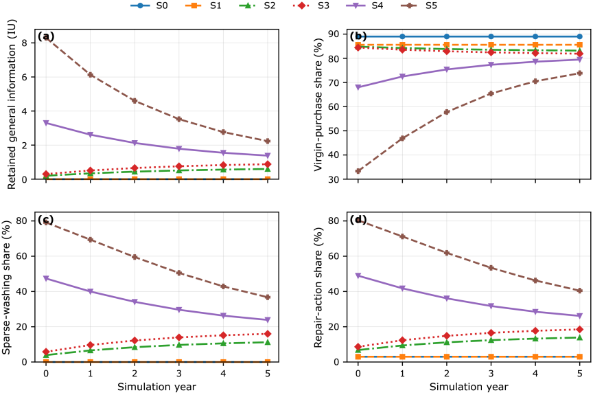
Fig. 2. Behavioural dynamics across the S0–S5 main scenario programme (Y0–Y5).
S2 and S3 contain recurring communication and therefore develop gradually rather than as one-time shifts. In S2, annual membership communication increases the retained general-information stock from 0.20 IU at Y0 to 0.60 IU at Y5. Over the same period, the sparse-washing share rises from 3.9% to 11.2%, the repair-action share from 6.8% to 13.9%, and the virgin-purchase share decreases from 84.8% to 83.2%. S3 adds garment-specific information, with one information view generated per expected wash. Its retained information increases from 0.30 IU at Y0 to 0.88 IU at Y5; sparse washing increases from 5.8% to 16.0%, repair from 8.6% to 18.5%, and the virgin-purchase share decreases from 84.4% to 81.9%. The S2 and S3 trajectories therefore show the accumulation of recurring communication under the two-year information half-life and the endogenous wash-linked exposure rule.
S4 and S5 have a different temporal profile because they include one-time education inputs at Y0. S4 starts at 3.30 IU of general information and S5 at 8.30 IU; these initial stocks subsequently decay while recurring membership and garment communication continue. Correspondingly, S4 sparse-washing and repair shares decrease from 47.4% and 48.9% at Y0 to 23.9% and 26.1% at Y5. S5 starts at 79.1% sparse washing and 80.4% repair and decreases to 36.7% and 40.5% at Y5. The S5 virgin-purchase share rises from 33.3% at Y0 to 73.8% at Y5 as the one-time education effect decays. This movement is an intended consequence of the time-dependent state equations, not an instability in the simulation: the interventions in S4 and S5 deliberately combine transient education with recurring communication, while S5 additionally retains the economic-incentive term.
The panels in Fig. 2 show retained general information [IU], virgin-purchase share [%], sparse-washing share [%], and repair-action share [%]. S0 and S1 are stationary because they contain no retained general-information input; S2 and S3 accumulate recurring communication; S4 and S5 begin with one-time education inputs that subsequently decay according to Eq. (4). Lines are expected-population results for \(N=\textrm{5,000}\) and are conditional model outputs rather than empirical response trajectories.
5.2. Propagation to Circular-System, Climate, and Cost Outcomes
The behavioural changes propagate through the interface described in Section 3.4 to the physical circular-system, life-cycle-impact and cost calculations. Table 3 gives the year-5 endpoints of all six main scenarios. The results form a consistent progression across the intervention ladder: lower virgin-purchase shares are accompanied by lower total denim requirements, non-decreasing effective lifetime, and lower calculated \(\mathrm{GWP}_{100}\) and allocated cost. The table reports calculated outputs, not additional scenario assumptions.
| Scenario | Virgin purchase [%] | Sparse wash [%] | Repair [%] | Lifetime [years] | Denim required [t] | \(\mathrm{GWP}_{100}\) [kt CO\(_2\)-eq] | Cost [million €] |
| S0 | 89.0 | 0.0 | 3.0 | 5.06 | 590.6 | 16.96 | 58.09 |
| S1 | 85.6 | 0.0 | 3.0 | 5.06 | 568.1 | 16.42 | 56.10 |
| S2 | 83.2 | 11.2 | 13.9 | 5.29 | 551.9 | 15.98 | 54.54 |
| S3 | 81.9 | 16.0 | 18.5 | 5.38 | 543.6 | 15.75 | 53.75 |
| S4 | 79.5 | 23.9 | 26.1 | 5.54 | 527.4 | 15.33 | 52.22 |
| S5 | 73.8 | 36.7 | 40.5 | 5.84 | 489.9 | 14.37 | 48.76 |
At Y5, S0 requires 590.6 t of denim, has a virgin-purchase share of 89.0%, produces 16.96 kt CO\(_2\)-eq of total \(\mathrm{GWP}_{100}\), and has an allocated cost of €58.09 million. The corresponding S5 values are 489.9 t, 73.8%, 14.37 kt CO\(_2\)-eq, and €48.76 million. Relative to S0, this is a reduction of 100.7 t of total denim requirement (17.0%), 15.2 percentage points in the virgin-purchase share, 2.60 kt CO\(_2\)-eq of total \(\mathrm{GWP}_{100}\) (15.3%), and €9.34 million of allocated cost (16.1%). Effective lifetime increases from 5.06 to 5.84 years, while recirculated denim used increases from 30.9 to 35.8 t.
The intermediate scenarios help identify where these changes enter the system. S1 isolates the purchase-decision channel: its point-of-purchase information changes the mix of virgin and circular purchase alternatives without changing the use-phase sparse-washing or repair probabilities. S2–S5 additionally alter retained information and therefore the use-phase and post-use routing variables. At Y5, the correct-sorting/recycling probability rises from 58.0% in S0 and S1 to 60.9% in S2, 62.2% in S3, 64.4% in S4, and 68.7% in S5. Across the same sequence, recirculated denim used rises from 30.9 t to 35.8 t. The result therefore reflects several linked mechanisms—purchase substitution, use-phase behaviour, lifetime, and post-use routing—rather than a direct mathematical effect of an information parameter on \(\mathrm{GWP}_{100}\) or cost.
The panels in Fig. 3 show virgin-purchase share [%], total denim required [t], total \(\mathrm{GWP}_{100}\) [kt CO\(_2\)-eq], and total allocated cost [million €]. The endpoints are calculated from the behavioural outputs through the unchanged circular-system, LCA, and cost equations. The scenarios are illustrative intervention conditions rather than estimated real-world policy effects.
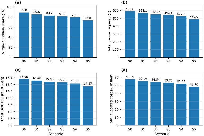
Fig. 3. Year-5 circular-system outcomes for S0–S5.
5.3. Sensitivity and Realised-Action Implementation Reproducibility Check
The one-at-a-time sensitivity programme contains 12 entries in four three-point families. In each family, the central point is the reference condition and is not counted as an independent sensitivity result: \(h=2\) years and \(\beta \times 1.0\) reproduce the S3–Y5 main-scenario result, whereas \(E=0.1\) and \(\Delta L_{\mathrm{repair}}=2\) years reproduce S5–Y5. Fig. 4 summarises deviations from these within-family references; the complete numerical results are provided in Additional Material S1.
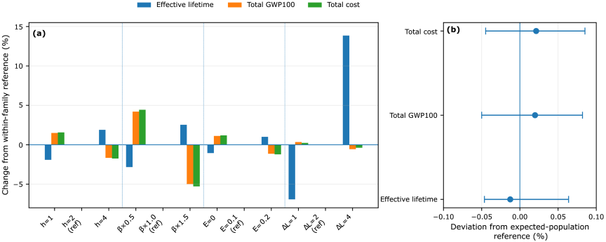
Fig. 4. One-at-a-time sensitivity and five-seed realised-action implementation reproducibility check.
The information half-life changes the persistence of recurring information in S3. Reducing the half-life from 2 to 1 year decreases effective lifetime by 1.91% and increases total \(\mathrm{GWP}_{100}\) and cost by 1.50% and 1.56%, respectively, relative to the S3–Y5 reference result. Increasing the half-life to four years increases effective lifetime by 1.89% and decreases \(\mathrm{GWP}_{100}\) by 1.66% and cost by 1.75%. The \(\beta\) sensitivity changes all non-zero information-response coefficients in S3. At \(\beta \times 0.5\), effective lifetime decreases by 2.83%, while \(\mathrm{GWP}_{100}\) and cost increase by 4.20% and 4.44%. At \(\beta \times 1.5\), effective lifetime increases by 2.54%, while \(\mathrm{GWP}_{100}\) and cost decrease by 4.98% and 5.28%. Among the tested behavioural-response sensitivities, \(\beta\) therefore produces the largest changes in the reported \(\mathrm{GWP}_{100}\) and cost outputs.
The S5 economic-intensity sensitivity produces smaller but directionally consistent changes. Removing the economic-incentive input (\(E=0\)) decreases effective lifetime by 1.06% and increases \(\mathrm{GWP}_{100}\) by 1.12% and cost by 1.19% relative to \(E=0.1\). Increasing \(E\) to 0.2 increases effective lifetime by 1.00% and decreases \(\mathrm{GWP}_{100}\) by 1.14% and cost by 1.22%. The repair-lifetime family tests a different type of uncertainty: it changes the physical lifetime consequence of an already-modelled repair action without changing the behavioural probabilities. With one additional year per repair, effective lifetime is 6.93% below the \(\Delta L_{\mathrm{repair}} = 2\)-year reference; with four additional years it is 13.86% above the reference. Total denim requirement is unchanged in this test, while downstream recirculated-denim, \(\mathrm{GWP}_{100}\), and cost quantities change through the effective-lifetime calculation. This distinction is useful because it separates uncertainty in behavioural response from uncertainty in the physical consequence assigned to a behaviour.
The five realised-action S5–Y5 runs with \(N=\textrm{5,000}\) and pseudorandom-number seeds 1729–1733 provide a separate implementation reproducibility check. All five runs satisfied the pre-specified implementation checks. Relative to the corresponding expected-population result, the mean deviations were \(+\)0.0199% for total \(\mathrm{GWP}_{100}\) and \(+\)0.0213% for total cost. Effective lifetime averaged 5.8390 years compared with 5.8398 years in the expected-population result and ranged from 5.8371 to 5.8435 years. The corresponding \(\mathrm{GWP}_{100}\) range was approximately \(-\)0.050% to \(+\)0.082% of the expected result and the cost range \(-\)0.045% to \(+\)0.085%. These small deviations show that the realised-action implementation behaves consistently around the expected-population calculation for the tested population size and seeds. They do not provide empirical validation of the behavioural assumptions.
In Fig. 4 (left), percentage change from the within-family reference for effective lifetime, total \(\mathrm{GWP}_{100}\), and total cost; \(h\) and \(\beta\) sensitivities use S3 at Y5 as their reference (\({h = 2}\) years and \({\beta \times 1.0}\)), whereas economic-intensity and repair-lifetime sensitivities use S5 at Y5 (\({E = 0.1}\) and \({\Delta L_{\mathrm{repair}} = 2}\) years). In Fig. 4 (right), mean and min-max deviation of five realised-action S5–Y5 runs (\({N=\textrm{5,000}}\); pseudorandom-number seeds 1729–1733) from the corresponding expected-population result. The central sensitivity points are references only; the realised-action runs test implementation reproducibility rather than empirical validity.
Taken together, the main scenario programme demonstrates the complete propagation chain implemented in the model: intervention conditions alter information and economic inputs; these alter agent-level decision probabilities; the aggregated decisions alter lifetime and circular-flow routing; and the downstream calculations alter material demand, \(\mathrm{GWP}_{100}\), and cost. The sensitivity programme shows that the magnitude of this propagation depends on explicit behavioural and physical assumptions, while the realised-action implementation check shows that sampled actions reproduce the expected-population result closely for the tested configuration. The methodological and practical implications, limitations and empirical calibration needs are discussed in Section 6.
6. Discussion
The significance of the results lies less in the numerical magnitude of the denim scenarios, which is conditional on the assumptions in Section 4, than in the demonstrated modelling chain. LCA scenarios often treat behaviour as a fixed assumption, while behavioural simulations do not necessarily resolve consequences in physical product systems 7,8,9,10,11,12,23. Here, interventions, heterogeneous response, decay, and physical flows are coupled in one calculable system, enabling pre-implementation testing and exposing which behavioural and physical parameters require empirical calibration.
At a broader scale, this suggests a shift in how circular-economy production is framed. Circularity cannot be scaled only by improving primary manufacturing while use and post-use decisions remain outside the production system. Continued use, maintenance, repair, redistribution, refurbishment, remanufacturing, component recovery, and recycling must instead become productive economic activities.
We use post-manufacturing production for this complementary domain: it does not replace manufacturing but extends production control and value creation beyond first sale into activities that the linear make-use-waste model largely treats as consumption and waste.
Under this perspective, economic activity and the services obtained from consumption need not scale in proportion to virgin production. Value creation can increasingly arise from keeping products functional, circulating and useful. The relevant scaling variable would therefore shift from the number of newly manufactured units towards the service and value obtained from material stocks already in circulation. This requires coordinated business models, service capacity, information infrastructures, and consumer participation. The present model offers one way to explore such coordination before implementation.
This economy-wide interpretation is a research direction, not a result established by the denim case. Generalisation requires empirical calibration of information acquisition, action and retention/decay across product and consumer contexts, and extension to interacting product systems, capacity constraints, rebound effects, distributional consequences, and policy conditions. If these steps are achieved, post-manufacturing production could become a calculable design layer for scaling circular-economy systems, allowing manufacturing and post-manufacturing production jointly to determine how much service and value can be generated per unit of virgin resource input.
7. Conclusion
Post-manufacturing production provides a perspective in which CE performance depends not only on product design and manufacturing, but also on the business model and on the decisions that determine what happens after a product has entered the market. For such responsibility to be exercised, economic operators need ways to communicate relevant information and incentives at the consumer decision points that influence acquisition, continued use, repair, handover, and post-use routing. The paper does not prescribe the communication infrastructure; this may combine customer-relations services with product-information infrastructures such as digital product passports.
By considering the circular business model and its associated value network as a post-manufacturing production system, a company may approach the incentivisation system for their customers with the same mindset as when increasing their manufacturing system efficiency and effectiveness. The economic operator can identify key circularity decisions, assess their potential influence on product lifetime and resource circulation, and test how different information and incentive configurations change the probability of those decisions. Consumer relations may range from broad brand-level awareness to repeated or event-triggered information linked to a product, service or specific action.
The key contribution of this work is therefore not only the integration of behaviour into LCA, but the ability to treat consumer incentives as controllable variables within a system model, enabling pre-implementation evaluation of behavioural strategies alongside technical and business model design. The denim case demonstrates this propagation from intervention conditions through probabilistic decisions to product lifetime, material flows, calculated \(\mathrm{GWP}_{100}\), and cost; the sensitivity analysis further shows that the magnitude of these outcomes depends explicitly on the behavioural-response and physical-link assumptions.
To assess and calibrate such interventions, empirical studies can be targeted at the specific quantities required by the model: information acquisition, whether awareness- or action-targeted information is actually received and registered by consumers; action, the probability of the intended behaviour following exposure; and retention/decay, how awareness and action propensity persist or diminish over time. These responses can be measured for different information types, delivery contexts and frequencies, including point-of-purchase, recurring, event-triggered, and educational communication. In this way, the simulation identifies which consumer-response parameters matter for circular-system performance, while targeted empirical studies provide the observations needed to calibrate them.
Accordingly, circular product designs and circular business models can be simulated across plausible levels of consumer participation before implementation, and observed outcomes can subsequently be compared with the simulation to refine the parameterisation. The model thereby treats consumer behaviour neither as a fixed external uncertainty nor as a fully controllable quantity, but as a heterogeneous, probabilistic and empirically calibratable component of circular-system performance. Low response levels or strong decay identified through calibration indicate where additional behavioural or system-level interventions are required.
Acknowledgments
The authors would like to thank the Swedish innovation agency Vinnova for their funding of the Visibility of Value Networks for Circularity and Eco-efficiency (VIVACE) project, grant number 2023-00868, as well as the Swedish governmental research council for sustainable development (Formas) who has provided funds for a deeper continuation into this field (grant number 2026-00357).
Footnotes
(1) Costs is roughly estimated as energy costs throughout the life cycle of materials and transports. This is justified by energy costs for extraction, enrichment, processing and transport. By improved cost and revenue models better comparisons between different actions may be achieved.
(2) Additional Material S1: IJAT_PIA_v0.6_Supplementary_Data.xlsx; SHA-256 checksum: 2a5904ad05bf4846f310b72254f8e64447323b56cb8be9b1c8a4065f16012d94; available at https://doi.org/10.5281/zenodo.22795205 [Accessed October 20, 2026].
- [1] S. Lang, G. Minnucci, M. Mueller, and M. P. Schlaile, “The role of consumers in business model innovations for a sustainable circular bioeconomy,” Sustainability, Vol.15, No.12, Article No.9573, 2023. https://doi.org/10.3390/su15129573
- [2] R. van den Berge, L. Magnier, and R. Mugge, “Sparking the repair ‘can-do’ attitude: Enhancing users’ willingness to repair through design support in fault diagnostics,” Int. J. Des., Vol.17, No.3, pp. 25-39, 2023. https://doi.org/10.57698/v17i3.02
- [3] L. Torca-Adell, P. Juan, and M. D. Bovea, “Exploring the acquisition, usage, repair, and end-of-life management practices of electrical self-care appliances: Insights from domestic and professional users,” Clean. Responsible Consum., Vol.16, Article No.100236, 2025. https://doi.org/10.1016/j.clrc.2024.100236
- [4] J. Camacho-Otero, C. Boks, and I. N. Pettersen, “Consumption in the circular economy: A literature review,” Sustainability, Vol.10, No.8, Article No.2758, 2018. https://doi.org/10.3390/su10082758
- [5] J. Kirchherr et al., “Barriers to the circular economy: Evidence from the European Union (EU),” Ecol. Econ., Vol.150, pp. 264-272, 2018. https://doi.org/10.1016/j.ecolecon.2018.04.028
- [6] R. Elzinga, D. Reike, S. O. Negro, and W. P. C. Boon, “Consumer acceptance of circular business models,” J. Clean. Prod., Vol.254, Article No.119988, 2020. https://doi.org/10.1016/j.jclepro.2020.119988
- [7] B. Corona, V. S. C. Tunn, and K. L. van den Broek, “Integrating consumer behaviour into the environmental assessment of circular packaging: A scoping review,” Int. J. Life Cycle Assess., Vol.29, No.1, pp. 430-447, 2024. https://doi.org/10.1007/s11367-023-02218-1
- [8] M. Lieder, F. M. A. Asif, and A. Rashid, “Towards circular economy implementation: An agent-based simulation approach for business model changes,” Auton. Agents Multi-Agent Syst., Vol.31, No.6, pp. 1377-1402, 2017. https://doi.org/10.1007/s10458-017-9365-9
- [9] M. Rizzati and M. Landoni, “A systematic review of agent-based modelling in the circular economy: Insights towards a general model,” Struct. Change Econ. Dyn., Vol.69, pp. 617-631, 2024. https://doi.org/10.1016/j.strueco.2024.03.013
- [10] R. Koide, H. Yamamoto, K. Nansai, and S. Murakami, “Agent-based model for assessment of multiple circular economy strategies: Quantifying product-service diffusion, circularity, and sustainability,” Resour. Conserv. Recycl., Vol.199, Article No.107216, 2023. https://doi.org/10.1016/j.resconrec.2023.107216
- [11] A. Micolier, P. Loubet, F. Taillandier, and G. Sonnemann, “To what extent can agent-based modelling enhance a life cycle assessment? Answers based on a literature review,” J. Clean. Prod., Vol.239, Article No.118123, 2019. https://doi.org/10.1016/j.jclepro.2019.118123
- [12] C. Davis, I. Nikolić, and G. P. J. Dijkema, “Integration of life cycle assessment into agent-based modeling: Toward informed decisions on evolving infrastructure systems,” J. Ind. Ecol., Vol.13, No.2, pp. 306-325, 2009. https://doi.org/10.1111/j.1530-9290.2009.00122.x
- [13] International Organization for Standardization (ISO), “Environmental management – Life cycle assessment – Principles and framework,” ISO 14040:2006, 2006. https://www.iso.org/standard/37456.html [Accessed October 20, 2026]
- [14] ISO, “Environmental management – Life cycle assessment – Requirements and guidelines,” ISO 14044:2006, 2006. https://www.iso.org/standard/38498.html [Accessed October 20, 2026]
- [15] ISO, “Circular economy – Measuring and assessing circularity performance,” ISO 59020:2024, 2024. https://www.iso.org/standard/80650.html [Accessed October 20, 2026]
- [16] R. S. Atlason, D. Giacalone, and K. Parajuly, “Product design in the circular economy: Users’ perception of end-of-life scenarios for electrical and electronic appliances,” J. Clean. Prod., Vol.168, pp. 1059-1069, 2017. https://doi.org/10.1016/j.jclepro.2017.09.082
- [17] T. G. B. Teixeira, J. F. de Medeiros, C. Kolling, J. L. D. Ribeiro, and D. Morea, “Redesign in the textile industry: Proposal of a methodology for the insertion of circular thinking in product development processes,” J. Clean. Prod., Vol.397, Article No.136588, 2023. https://doi.org/10.1016/j.jclepro.2023.136588
- [18] B. Pozo Arcos, C. Bakker, and R. Balkenende, “How user manuals support the diagnosis of common faults in household appliances: An analysis of 150 manuals,” Circ. Econ. Sustain., Vol.3, No.1, pp. 535-555, 2023. https://doi.org/10.1007/s43615-022-00195-5
- [19] S. Lawrenz et al., “Implementing the circular economy by tracing the sustainable impact,” Int. J. Environ. Res. Public Health, Vol.18, No.21, Article No.11316, 2021. https://doi.org/10.3390/ijerph182111316
- [20] A. Taron, A. Majumder, S. Bodach, and D. Agbefu, “Public-private partnerships for the circular bio-economy in the Global South: Lessons learned,” Resource Recovery and Reuse Series, No.22, International Water Management Institute, 2023. https://doi.org/10.5337/2023.205
- [21] P. K. Mallick, K. B. Salling, D. C. A. Pigosso, and T. C. McAloone, “Towards a circular economy: Development of a support tool for designing reverse logistics systems,” J. Environ. Manage., Vol.351, Article No.119819, 2023. https://doi.org/10.1016/j.jenvman.2023.119819
- [22] V. Ramani and P. De Giovanni, “Circular economy business strategies and public schemes: A game theory-based survey,” Int. Trans. Oper. Res., Vol.33, No.5, pp. 2827-2869, 2026. https://doi.org/10.1111/itor.70031
- [23] J. Walzberg, J.-M. Frayret, A. L. Eberle, A. Carpenter, and G. Heath, “Agent-based modeling and simulation for the circular economy: Lessons learned and path forward,” J. Ind. Ecol., Vol.27, No.5, pp. 1227-1238, 2023. https://doi.org/10.1111/jiec.13423
- [24] E. G. Gulserliler, J. D. Blackburn, and L. N. Van Wassenhove, “Consumer acceptance of circular business models and potential effects on economic performance: The case of washing machines,” J. Ind. Ecol., Vol.26, No.2, pp. 509-521, 2022. https://doi.org/10.1111/jiec.13202
- [25] European Parliament and Council of the European Union, “Regulation (EU) 2024/1781 establishing a framework for the setting of ecodesign requirements for sustainable products,” 2024. http://data.europa.eu/eli/reg/2024/1781/oj [Accessed October 20, 2026]
- [26] European Committee for Standardization and European Committee for Electrotechnical Standardization (CEN-CENELEC), “CEN/CLC/JTC 24 – Digital product passport – Framework and system.” https://standards.cencenelec.eu/dyn/www/f?p=205:7:0::::FSP_ORG_ID:3342699&cs=1798F43FAA14922B642266F24B912DC61 [Accessed October 20, 2026]
Appendix
Appendix A. The Post-Manufacturing Production
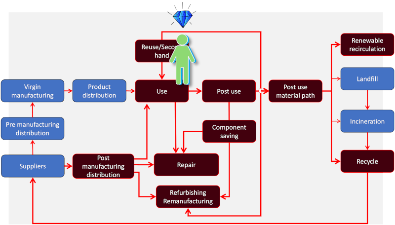
Figure 5 represents the circular system presented in Fig. 1 in Section 3. The post-manufacturing production system represents all parts enabling the circular functions and performance of the production system, such as prolonged lifetime, reuse, repurpose, remanufacturing, recycling, renewable recirculation (regeneration), etc. The methodology described in Section 3 establishes agents that represent consumers at core points around the Use-phase in this model to run different scenarios of how different information strategies may impact the decisions that consumers make, and how these decisions impact the material flows between the different process boxes. The changes in material flows result in environmental and economic consequences of the whole production system, as presented in Section 5.
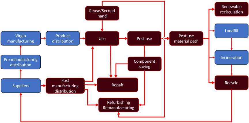
Fig. 5. The post-manufacturing production system (bourgogne process boxes) in a total circular production system context.
This article is published under a Creative Commons Attribution-NoDerivatives 4.0 Internationa License.