
Research Paper:
Real-Time Estimation of Temperature Field and Thermal Displacement in Machine Tool Linear Motion Systems Using Servo Data
Ryoji Kondo*,† and Kazuhito Ohashi**

*YASDA PRECISION TOOLS K.K.
1160 Hamanaka, Satosho-cho, Asakuchi-gun, Okayama 719-0303, Japan
†Corresponding author
**Faculty of Environmental, Life, Natural Science and Technology, Okayama University
Okayama, Japan

Heat generated in machine tools during operation causes thermal deformation and deteriorates machining accuracy. To suppress thermal deformation and the resulting displacement, strategies such as reducing heat generation, cooling machine elements that generate heat, and compensating for thermal displacement are generally adopted. However, existing methods for estimating and compensating for thermal deformation and displacement can only be adopted in limited situations. In particular, there are few reports on real-time estimation methods that take into account moving parts and actual machine operating conditions. For high-accuracy machining, it is important to understand the temperature field and the associated displacement. In this study, real-time estimation of the temperature field and displacement is carried out on a test apparatus equipped with a ball screw drive system and a linear guideway system. In the estimation process, heat generation values are first calculated from servo data corresponding to the machine operation. Using these calculated values, the temperature field is then derived through the finite volume method. Finally, the thermal displacement is obtained from the temperature field using a simplified estimation method. The results are validated by comparison with experimental data and with results from commercial finite element method software, demonstrating the effectiveness and real-time performance of the proposed approach.
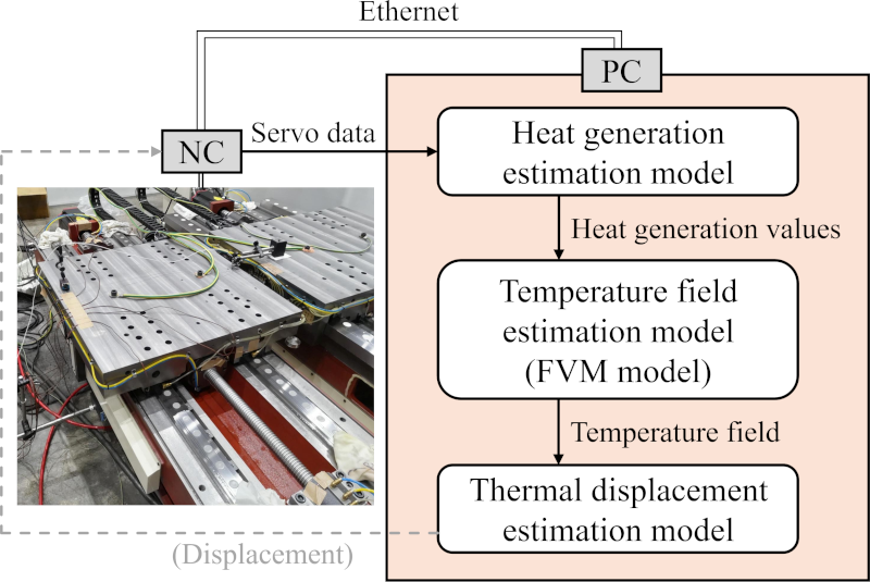
Procedure for estimating temperature field and thermal displacement
1. Introduction
The effects of internal and external heat sources on machine tools cause thermal deformation, leading to a deterioration of machining accuracy. Peripheral devices, such as hydraulic units and electrical units, which are classified as external heat sources, can be thermally insulated to mitigate the machine’s thermal deformation. On the other hand, main machine elements classified as internal heat sources, such as spindles, ball screws, motors, and bearings, are responsible for the machine’s performance. Thus, it is more difficult to suppress the effects of these heat sources on thermal deformation without degrading the machine’s performance. In general, reducing heat generation, cooling heat-generating elements 1,2,3,4,5, and applying compensation methods 6,7,8,9,10,11 are adopted as countermeasures to suppress the machine’s thermal deformation. In recent years, there have been many reports on estimation and compensation methods for thermal deformation using machine learning, surrogate models, adaptive learning control, and neural networks 12,13,14,15,16,17,18.
However, those estimation methods can only be used in limited situations. For example, they may consider only a part of a machine tool, such as the spindle or the column, use fixed values for heat generation, focus solely on ambient temperature changes, or require information obtained from external sensors, etc. There have been few reports that take into account the effects of moving parts in the estimation of and compensation for thermal displacement. When the finite element method (FEM) is used to estimate the temperature field and thermal displacement, the computational cost tends to be high, which prevents real-time estimation or compensation. In this study, the authors propose methods to estimate the temperature field and the thermal displacement of a test apparatus with a ball screw drive system and a linear guideway system without time-consuming calculations or loss of real-time performance.
In general, thermal deformation caused by the operation of machine tools is not a rapid phenomenon. Although it depends on the rate at which the displacement to be estimated and compensated occurs, the thermal displacement induced by the operation of linear feed axes is considered to be relatively small. Therefore, it was assumed that if estimation and compensation can be performed on a cycle of several minutes, displacements that would become problematic in typical machine tool operations can be sufficiently suppressed.
In this study, a personal computer (PC), connected to the machine controller via Ethernet, acquired servo data including position and current values corresponding to the actual machine operation at fixed time intervals. Heat generation in each machine element assumed to be a heat source was calculated using an estimation model, and the finite volume method (FVM) was applied with these values to estimate the temperature field. Then, the FEM analysis of only the ball screw shaft and the table was performed based on the temperature field, and the displacement at the top surface of the table was estimated. The obtained temperatures and displacement were compared with experimental results and with results from commercial FEM software to verify the performance.
2. Experimental Procedures and Conditions
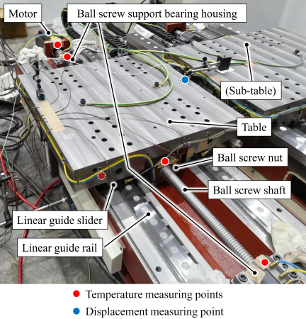
Fig. 1. Overview of the test apparatus.
Figure 1 shows the test apparatus used in the study. The apparatus is a single-axis linear feed system with a ball screw drive system and a linear guideway system installed in a temperature-controlled room. Its structure is equivalent to that of the actual table axis of a machining center. The stroke is 900 mm. A constant amount of lubricating oil (VG68) is supplied at fixed intervals to the ball screw nut, the ball screw support bearings, and the linear guide sliders. This apparatus is equipped with a cooling circuit for the ball screw nut and the ball screw support bearings; however, the cooling function was not used in this study.
Table 1 summarizes the experimental conditions. There were three feed rate conditions, and the reciprocating motion was repeated for 200 min. The ball screw nut is 170 mm long, and the travel distance is 16 mm, which is short enough compared with the length of the ball screw nut. The commercial FEM software (Creo Simulate, PTC) used in this study cannot simulate heat generation with movement of parts. To simulate the experimental situation with this software, the travel distance was set small enough to generate heat without causing failure of the ball screw. Servo data of the table’s position and the motor’s current value were acquired by a PC connected to the machine controller (Fanuc) via Ethernet at a sampling rate of 1 ms. After reciprocating five times, there was an additional dwell time for outputting the servo data during the machine operation to a CSV file.
The temperatures of the motor bracket, the ball screw support bearing housings, the ball screw nut, and the linear guide sliders were measured using T-type thermocouples. In addition, the ambient temperature was measured to confirm that the room temperature was stable during operation. The displacement of the tabletop surface, which directly affects the machining accuracy, was measured using a capacitive displacement sensor (CPL290, Lion Precision). The displacement sensor was held by a magnetic stand placed on the tabletop surface of another test apparatus (sub-table) installed next to the test apparatus used in this study. The sub-table was not operated during the experiment. The data logger (NR-500, Keyence) acquired the temperatures and displacement with resolutions of 0.01°C and 0.4 nm, respectively, and the sampling rate was set to be 1 s. The displacement measurement is affected by the target surface profile; thus, the data obtained while the table was stopped were extracted as the displacement data. Before the machine operation, the machine was left for a sufficient time with the power on.
| Feed rate [mm/min] | 3000, 5000, 10000 |
| Travel distance [mm] | 16 |
| Operation cycle |
|
| Operation time [min] | 200 |
| Temperature measurement |
|
| Displacement measurement | Tabletop surface |
| Sampling rate [s] | 1 |
| Resolution | 0.01°C (temperature) 0.4 nm (displacement) |
3. Estimation Methods of Temperature Field and Thermal Displacement
Figure 2 shows an overview of the real-time estimation method. First, we determine the heat generation values of each part based on the servo data mentioned above and use a heat generation estimation model. Next, the heat generation values are applied to the FVM model prepared in advance, and the temperature field is obtained by solving the simultaneous equations. Then, the displacement is estimated based on the temperature field using a thermal displacement estimation model. To conduct this algorithm, we created programs to acquire servo data, estimate the heat generation values, solve the FVM, and estimate the thermal displacement. The program to acquire the servo data was written in C++, and all other programs were written in Python.
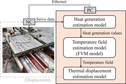
Fig. 2. Procedure for estimating temperature field and thermal displacement.
3.1. FVM Model and Thermal Displacement Estimation Model
We used the FVM model to simulate the temperature field and briefly describe the theory here. Fig. 3 is a 2D diagram that shows an overview of the FVM used in this study. As a basic idea, the analytical area needs to be discretized into finite cells, and heat balance is considered at each cell. Then, the heat balance is thought to lead to a temperature change in each cell. By formulating the equations for each cell and solving these equations as simultaneous equations, we can obtain the temperatures of all cells, i.e., the temperature field. The temperature change in this study is not large; thus, we assume that the effect of radiative heat can be ignored. Therefore, in this case, we should consider the effects of heat conduction, convective heat transfer, and heat generation. Thermal contact resistance depends on surface characteristics and contact conditions; however, identifying these individually in an actual machine is generally impractical, and thus it is not considered in this study. Heat exchange occurs at the surface of the cell, and we set up generalized equations that consider heat conduction, convective heat transfer, and heat generation. Regarding heat conduction, we assume that the temperature is defined at the center of gravity and that the heat conduction occurs between these centers. The amount of heat conduction for a time \({\Delta}t\) is expressed as follows:
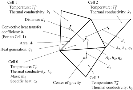
Fig. 3. Conceptual diagram of FVM adopted in this study.
Here, the subscript \(i\) (\(i=1\)–\(3\) in the diagram) denotes the index of the element or the surface adjacent to cell 0, \(k_{i}\) is the thermal conductivity, \(d_{i}\) is the distance between the centers of gravity, \(T_{i}^{n}\) is the temperature of the cells at time step \(n\), and \(A_{i}\) is the surface area where heat conduction, heat transfer, or heat generation occurs. The thermal conductivity is determined by the physical properties of the cells in which heat conduction occurs. In this study, we used the harmonic mean of thermal conductivities. Strictly speaking, the line connecting the centers of gravity is not necessarily perpendicular to the heat conduction surface; however, we checked the quality of the cells and assumed that its effect on the error was small. Regarding heat transfer, the amount for a time \({\Delta}t\) is expressed as follows:
Here, \(h_{i}\) is the heat transfer coefficient, and \(T_{a}\) is the temperature of the room air. The relative wind speed on the surfaces except the ball screw is not sufficiently high to significantly affect the heat transfer coefficient, so the heat transfer coefficient value corresponding to still air, 7 W/(m\(^{2}\)K), was adopted for those surfaces. The heat transfer coefficient on the ball screw surface is considered to be slightly higher than that for still air. We determined these values by considering the proportion of time spent stopping and moving in each feed rate condition 19. The heat generation values were determined from the values per unit area and time, the surface areas, and the time, as expressed as follows:
Here, \(q_{i}\) is the heat generation value per unit area and time, and \({\Delta}t\) is the time during which heat generation occurs. Considering the heat balance including the above values leads to a temperature change of the cell. At this point, the relation between the heat balance and the temperature change is expressed as follows:
Here, \(m_0\) is the mass of the cell, \(c_0\) is the specific heat capacity of the cell, and \({\Delta}T_0\) is the temperature change of the cell. Rearranging for \({\Delta}T_0\), we obtain
Transforming this into matrix form, we obtain
Here,
Setting \(k_{i}\) to 0, the heat transfer without heat conduction can be expressed, and the same applies to \(h_{i}\) and \(q_{i}\). As mentioned above, by creating the equations at each cell and solving them, the temperature field at time step \(n\) can be obtained. Each coefficient matrix element is assigned to the corresponding global matrix element. To solve the simultaneous equations, we use the LU decomposition which is a type of direct method, because once we perform the LU decomposition, we can use the decomposed matrices as long as the global matrix does not change. Focusing on Eq. (6), the heat generation values \(q_{i}\) appear only on the right-hand side. Assuming \(k_{i}\) and \(h_{i}\) are constant values, the global matrix does not change; therefore, we only need to update the right-hand-side vector to advance the time step, which is considered suitable for high-speed calculation. For cell discretization, Gmsh, an open-source 3D finite element mesh generator, was used in this study. The cell shape is tetrahedral to conform to the geometry. By extending this to three dimensions, the above idea can be applied to arbitrary shapes.
In the operation of actual machine tools, machining processes, cutting fluid, and chip accumulation result in highly complex phenomena, and it is not practical to account for all of these effects, including their observation. In this study, the focus is placed on a fundamental evaluation of machine operation, and the heat transfer coefficients and heat generation elements are fixed under each condition. Reconstructing the global matrix to account for temporal variations in these conditions would compromise real-time performance. Therefore, depending on the required computational speed, one possible approach is to prepare matrices corresponding to several representative conditions in advance and load and use them as needed for the computation. However, since the present study focuses on operation under a predefined cycle, this approach is not implemented.
It is considered difficult to calculate the displacement of the whole model by FEM on a general PC because the computational cost tends to be high and prevents real-time estimation. Therefore, we have to consider alternative estimation methods for thermal displacement. From the thermal deformation result obtained with Creo Simulate under the condition of 5000 mm/min, shown in Fig. 4 as a color contour map of total displacement, the main factors affecting the displacement of the tabletop surface are considered to be the convex deformation of the bed caused by the thermal elongation of the ball screw and the thermal deformation of the table. Therefore, we decided to use FEM only for the ball screw shaft and the table in order to obtain the thermal deformation of the bed and the table, respectively. The elements are linear tetrahedral elements shared with the cells of the FVM.
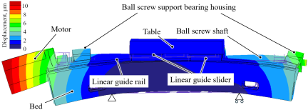
Fig. 4. Deformation result obtained with Creo Simulate under the condition of 5000 mm/min.
Regarding the convex deformation of the bed, we consider here the relationship between this deformation and the thermal elongation of the ball screw shaft. The temperature field of the ball screw shaft can be obtained using the FVM, and the thermal elongation of the shaft, when it is regarded as a cantilever beam, can also be obtained. The shaft is assumed to be compressed to its actual elongation as a double-sided beam. The force caused by the thermal elongation of the ball screw shaft can be calculated from the stiffnesses of the shaft and the structure supporting the shaft. This yields a simple statically indeterminate problem expressed as follows:
Here, \(F\) is the force caused by the thermal elongation of the ball screw shaft, \(k_\mathit{bs}\) is the stiffness of the ball screw shaft in the axial direction, \(k_\textit{bed}\) is the stiffness of the bed in the axial direction, and \(x_\textit{cantilever}\) is the thermal elongation of the ball screw shaft in the case of a cantilever. In advance, the guide rail profile was measured when a 1 N force was applied to the ball screw support bearings, and, by multiplying this profile by the calculated force, the guide rail profile can be estimated as long as the response remains in the linear region. The ball screw is installed with preload by pulling one end, and the other end is structurally fixed. The fixed end (motor side) is set as the constraint condition, and the displacement of the other end (non-motor side) is calculated by FEM. The stiffness of the ball screw shaft and the bed, and the guide rail profile when a 1 N force is applied, were obtained using Creo Simulate. The table analysis was conducted with the linear guide sliders and the ball screw nut set as constraint conditions.
For comparison, the temperature field and the thermal deformation and displacement were simulated using Creo Simulate. Heat generation was assumed to occur at the motor, the ball screw support bearings, the ball screw nut, and the linear guide sliders.
Before considering the real-time estimation based on the servo data, we have to identify the heat generation values in the actual experiment for each feed rate condition. The machine operation repeats reciprocating motion including stopping and moving, and therefore, heat generation was assumed to occur intermittently; however, in this study, heat generation values corresponding to continuous heat generation were identified. Using the temperature changes of the actual experimental results as the target, the simulation was conducted repeatedly so that the simulation results matched the experimental results by inverse analysis. Since Creo Simulate is not efficient for repeating simulations, the FVM program we developed was used to identify the values. After identifying the values, simulations with Creo Simulate were conducted using these values.
3.2. Heat Generation Estimation Model Using Servo Data
The test apparatus used in the study has a FANUC controller, and the servo data can be acquired using the FOCAS library. The trigger command is written in the NC program. When the PC connected to the NC controller via Ethernet detects the trigger command, it starts to acquire the servo data every 1 ms for the specified sampling time and outputs the data to a CSV file. Then, the PC waits again until the trigger command is issued. Fig. 5 shows the time relationship in data acquisition. In this study, the data acquisition time was set to 14 s for one operation cycle at any feed rate condition. We have to set the data acquisition time in advance; thus, strictly speaking, this time is different from the actual machine operation time. In addition, the process of outputting a CSV file takes a few seconds. In other words, there are moments when data are not acquired while the PC outputs a CSV file and waits for the next trigger command. However, since the machine was stopped while the PC could not acquire the data, the missing data period was complemented by the data obtained while the machine was stopped. Then, the real-time estimation program is executed when it is detected that the CSV file has been output. We determined that the analysis time was 18 s for all feed rate conditions.
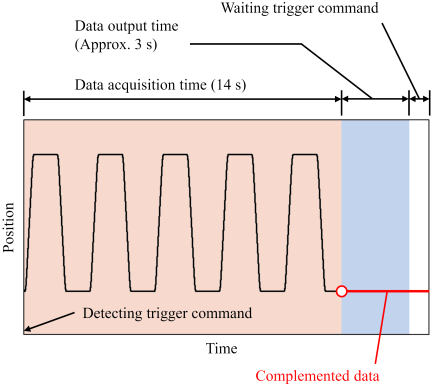
Fig. 5. Time relationship of data acquisition.
We consider here an estimation model of heat generation values from the servo data. We assume that the heat sources are the motor, the ball screw support bearings, the ball screw nut, and the linear guide sliders. There are two kinds of heat generation mechanisms: friction and motor loss. Regarding friction, the heat generation value is expressed as the product of the friction force and the velocity, and we assume that the heat generation is expressed as follows:
Here, \(N\) is the normal force, \({\mu}\) is the friction coefficient, \(\mu_V\) is the velocity-dependent coefficient of the friction coefficient, and \(v\) is the velocity. Above a certain velocity threshold, the friction coefficient is considered to be approximately proportional to velocity due to the viscosity of the lubricating oil. At low velocities, even if the friction coefficient exhibits nonlinear behavior, its influence on the frictional heat generation becomes sufficiently small because it is multiplied by velocity. This tendency is also supported by the data reported in the literature 20. Therefore, a linear model is adopted in this study. In the case of the ball screw nut and ball screw support bearings, the normal forces include the effects of inertia forces due to acceleration and deceleration. Regarding motor loss, we assume that the heat generation is proportional to the square of the motor current. To estimate the heat generation values, we have to identify parameters such as the friction coefficient, the velocity-dependent coefficient, and the motor loss coefficient. The motor loss coefficient is determined so that the simulation result for the motor matches the actual temperature change while the table is being pushed against the stopper. In this condition, current is supplied, and torque is generated, whereas the motor shaft does not rotate and frictional heat is not generated. Therefore, the effect of frictional heat in the bearings can be ignored, and the coefficient can be determined. The preliminary experiments were conducted separately from the main experiments, though under the same feed rate conditions. Using servo data from one operation cycle of these preliminary experiments at each feed rate condition, the heat generation values at each heat source were calculated. The servo data were sampled at 1 ms, and the velocity and acceleration were calculated from the position data. With these values, the heat generation values are calculated at every 1 ms, and then the sum is converted to a value per unit time. At each feed rate condition, equations were formulated by setting these calculated values equal to the values identified by the FVM program mentioned above as simultaneous equations, and by solving them, the parameters were determined.
In the real-time estimation, the heat generation values are updated at every operation cycle by recalculating them from the servo data and parameters determined above. The heat generating areas of the motor and the ball screw support bearings do not change depending on the operation, so only their heat generation values need to be updated. On the other hand, for the ball screw nut and the linear guide sliders, both the heat generation values and their distributions have to be updated because the table position changes from moment to moment during operation. Fig. 6 shows an overview of the implementation of this concept for the ball screw. The surfaces were divided into multiple areas along the axis, and the values per unit time were assigned to each area. In this study, the surface of the ball screw shaft over which the nut can move and the surfaces of the linear guide rails contacted by the sliders were divided into 200 areas; the lengths of each area were approximately 8 mm and 10 mm, respectively. The heat generation values are calculated at every 1 ms from the velocity, the acceleration, and the parameters determined above, and are added to the positions where the ball screw nut and the sliders are located at the moment over one cycle time. In the actual calculation, the values per unit area and per unit time are assigned to the surfaces of the cells included in each divided area. The heat generation values are calculated at every operation cycle; however, to improve the estimation accuracy, an additional calculation is conducted with a time step equal to one-tenth of the operation cycle time, because the FVM calculation can be performed rapidly. Therefore, the results calculated over ten time steps are output as the result for one operation cycle.
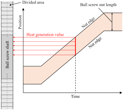
Fig. 6. Conceptual diagram of method for determining heat generation distribution based on time-position relationship of servo data.
A simulation model in which the relative position of the table and the bed does not change is not versatile. When the whole model including the table and the bed is used, the simulation can be adopted only to operations in which the travel distance is extremely limited, such as in the experiment in this study. However, performing calculations while changing the relative position of the table and the bed from moment to moment would require updating the global matrix at very high speed, which is impractical. Therefore, we treated the table and the bed as separate models and performed the calculations separately. There are six types of results to be compared; the experiment, Creo Simulate, the whole model including the bed and the table with fixed heat generation values and areas, the separate model under the same heat generation conditions, the whole model with real-time estimation, and the separate model with real-time estimation. Table 2 shows the details of the simulation models and conditions. The materials of the models are assumed to be cast iron and bearing steel, and their material properties are taken from the literature 21,22,23. The time step and mesh size used in this study were validated by conducting the same analysis with finer temporal and spatial discretization. As the results showed only minor differences in the quantities of interest, the adopted discretization was considered to provide sufficient accuracy.
| FVM | Cell shape | Tetrahedral | ||||
| Number of cells | Whole model: 100431, table: 25443, bed: 80755 | |||||
| Heat generation | Motor | |||||
| Ball screw support bearings (2 areas) | ||||||
| Ball screw nut | ||||||
| Linear guide sliders (4 areas) | ||||||
| Convective heat transfer coefficient [W/(m\(^2\)K)] | Ball screw shaft: | |||||
| 9.0 (3000 mm/min) | ||||||
| 9.0 (5000 mm/min) | ||||||
| 9.4 (10000 mm/min) | ||||||
| Other: 7.0 | ||||||
| FEM | Element shape | Linear tetrahedral | ||||
| Number of elements / nodes | Ball screw shaft: 5167 / 1905 | |||||
| Table: 25443 / 7174 | ||||||
| Restraint | Ball screw shaft: fixed end | |||||
| Table: linear guide sliders, ball screw nut | ||||||
| Load | Thermal stress based on temperature distribution | |||||
| Creo Simulate | Element shape | Tetrahedral | ||||
| Number of elements / nodes | 23802 / 7504 (\(p\)-adaptive) | |||||
| Heat generation [W/m\(^2\)] | Feed rate [mm/min] | 3000 | 5000 | 10000 | ||
| Motor | 120 | 175 | 460 | |||
| Ball screw support bearing (Motor side) | 260 | 315 | 405 | |||
| Ball screw support bearing (Non-motor side) | 300 | 363 | 480 | |||
| Ball screw nut | 55 | 75 | 100 | |||
| Linear guide sliders | 30 | 50 | 120 | |||
| Restraint | Bed supporting points (4 points) | |||||
| Load | Thermal stress based on temperature distribution | |||||
| Materials | Cast iron | Bed, table, ball screw support bearing housings | ||||
| Bearing steel | Motor, ball screw support bearings, ball screw shaft, ball screw nut, linear guide rails, linear guide sliders | |||||
4. General Features of FEM Software
Generally speaking, commercial FEM software, especially CAE tools for design engineers, is not intended to output results in real time. A model is prepared, simulation conditions are defined, and simulation time and output time steps are set in this process. Thereafter, the simulation is carried out, and the results are output when the simulation is completed. Thus, even if the calculation can be performed rapidly, it is not common to output results at every simulation time step and use them for compensation. Certainly, it may be possible to output the results at every time step using specific tools and knowledge. Nonetheless, it is difficult to perform simulations that include moving parts. In that case, the simulation has to be nonlinear analysis, and the global matrix has to be updated at each time step; accordingly, the computation time tends to be long. In addition, using external data, such as the servo data in this study, to simulate moving parts is not common.
Therefore, in this study, the simulation with Creo Simulate was conducted at a time completely separate from the experiment. The heat generation values and areas were fixed as simulation conditions, and the table motion was not considered in the simulation.
5. Comparison of Results from Experiments, Proposed Approach, and Commercial FEM Software
Figure 7 shows the experimental and simulation results of the temperature change and thermal displacement at the feed rates 3000, 5000, and 10000 mm/min. Figs. 7(a)–(f) show, respectively, the temperature changes of the motor bracket, the ball screw support bearing housings (motor side), the ball screw support bearing housings (non-motor side), the ball screw nut, the linear guide slider, and the displacement of the tabletop surface. The results of Creo Simulate, the whole model, and the separate model with fixed heat generation values and areas are plotted at 10 min intervals as one time step. In the thermal analysis of Creo Simulate, time steps can be interpolated to capture regions with steep changes; therefore, more data points are plotted than at 10 min intervals.
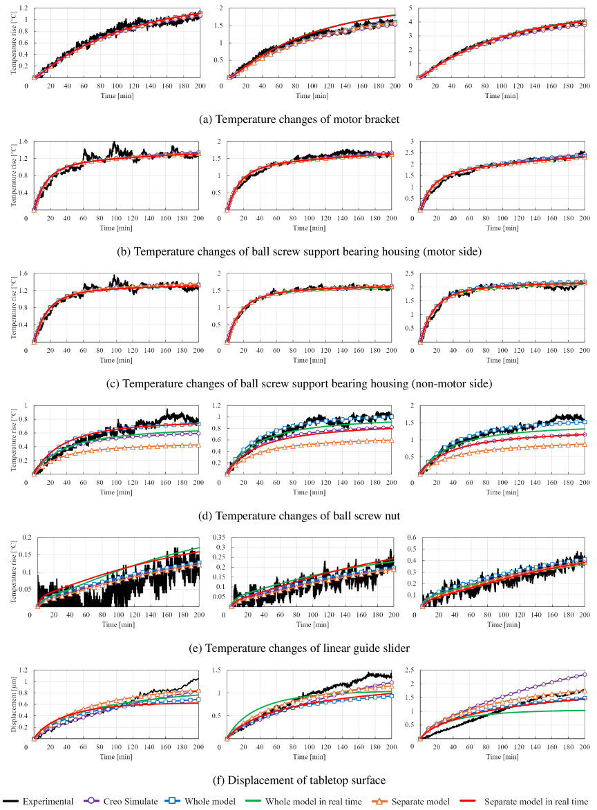
Fig. 7. Comparison of results from experiments, proposed approach, and commercial FEM software (from left to right: 3000 mm/min, 5000 mm/min, and 10000 mm/min).
Regarding the results of the whole model, the heat generation conditions were adjusted so that the temperature changes matched the experimental results, thus, the temperature changes, including the transient behavior, agreed well with the experiment, and the model is considered to be well replicated. The displacement did not agree with the experiment as well as the temperature changes because the displacement was obtained using a simple estimation method rather than FEM of the whole model. Regarding the results of Creo Simulate, the temperature changes agreed well with those of the experiment and the whole model, except at the ball screw nut. The heat generation conditions were the same as in the whole model; however, there may have been specific differences in the treatment of heat generation applied to inner surfaces. The displacement was relatively consistent with the experimental result; in particular, the time constants matched well, because FEM including both the table and the bed was performed.
In the case of the whole model with real-time estimation, the temperature changes of the motor and the ball screw support bearings agreed well with those of the whole model in which the heat generation values were fixed and not distributed. The results for the ball screw nut and the linear guide slider were also relatively consistent under all feed rate conditions. In this model, a single set of estimation parameters for the heat generation was used and was not changed depending on the feed rate condition; only the servo data used in the calculation were changed. From these results, the estimation parameters are considered to have been properly identified. Concerning the separate model, it is obvious that heat conduction between the ball screw shaft and nut and between the linear guide rails and sliders was not taken into account, simply because they were modeled separately. As a result, the temperature change of the ball screw nut was significantly lower than in the whole model. It is considered that, in the separate model, the temperature of the ball screw shaft tends to be higher than that of the nut, and that, in the whole model, heat conduction from the shaft to the nut occurs. In the separate model, there was no heat conduction; therefore, the temperature of the nut was lower, and the temperature of the shaft is thought to have been higher than in the whole model. The displacement result was larger than in the whole model, which also suggests that the temperature change of the ball screw shaft, leading to the deformation of the bed, was higher.
When using the separate model, we have to take heat conduction into account in some way. Therefore, we decided to use the temperatures of the cells that include the surfaces in the contact areas to simply account for heat conduction. In principle, heat conduction should be solved implicitly by considering the temperatures of all cells; however, that is difficult because the relative position of the table and the bed changes from moment to moment. It is considered that, as the time step of the simulation becomes longer, the simulation accuracy deteriorates. In this study, the thermal conduction analysis was carried out every 1.8 s, and we considered that the effect was not very significant and that a certain level of accuracy could be ensured. The heat conduction between the linear guide rails and sliders was less affected by separating the model; therefore, only the ball screw shaft and nut were treated in this way. The temperature of the nut was defined as a single value by averaging the temperatures of the cells. The surface of the shaft was already divided into multiple areas, and the average temperature of the cells was defined for each area. In the process of estimating the heat generation values, the durations of contact for each area were calculated, and these durations were used to calculate the heat conduction of each area. Regarding the results of the separate model with the real-time estimation taking heat conduction into account, the estimated temperature change of the nut, while not perfect, showed improved accuracy. In addition, the displacement was almost the same as that of the whole model without the real-time estimation; thus, it is considered that the temperature of the ball screw shaft was also simulated well.
Displacement without distribution, for instance, spindle thermal displacement, can be compensated by rewriting and updating the coordinate origin. For displacement with distribution, the compensation value depends on the position of moving parts such as the table. Therefore, we need to rewrite and update the coordinate origin rapidly or modify the operation program directly. However, at present there is no compensation function for such displacement, and it is difficult to compensate even if the distributed thermal displacement is known. In operations where the travel distance is short, such as in this experiment, the proposed methods can be adopted; otherwise, an alternative compensation function is required.
To consider the validity of the compensation using the real-time estimation proposed in this study, the experimental result was compared with the result obtained by subtracting the estimated value. In addition, the result obtained by subtracting the Creo Simulate result was also compared in terms of compensation accuracy and real-time performance. For the feed rate of 5000 mm/min, the thermal displacement and the simulation time from the start of the simulation to obtaining the results were compared. Fig. 8 shows the comparison results.
The result without compensation and the result with real-time compensation are plotted in the time-displacement plane. To compare the compensation accuracy, the result obtained by subtracting the Creo Simulate result is also plotted in the same plane in a lighter color. The simulation-time axis represents the time required for the simulation up to each time point. The real-time estimation method proposed in this study was executed on a laptop with an Intel™ Core i7-8650U CPU and 16 GB of RAM. Creo Simulate was executed on a PC with an Intel™ Xeon W-2135 CPU, an NVIDIA Quadro P4000 graphics board, and 64 GB of RAM.
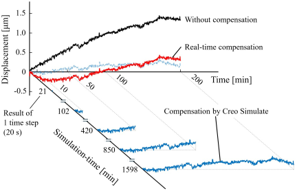
Fig. 8. Comparison of compensation accuracy and simulation time obtained using proposed approach and commercial FEM software at 5000 mm/min.
The maximum displacements relative to 0 μm for the cases without compensation, with real-time compensation, and with compensation using Creo Simulate were approximately 1.45, 0.44, and 0.34 μm, respectively. The displacement with real-time compensation was less than one third of that without compensation. The real-time estimation method requires less than 2 s from data reading to obtaining the results in each operation cycle. For comparison of simulation time, the simulation time step of Creo Simulate was set to 20 s, equivalent to the time step of the real-time estimation. Naturally, as the number of simulation steps increases, the required simulation time also increases. Even the simulation for a single time step takes approximately 21 min. Because the simulation process includes pre-processing and post-processing and there should be algorithms to ensure the accuracy of the analysis, the actual calculation time is different from the simulation time; however, it is considered infeasible to obtain results at the same speed as the real-time estimation method.
Based on the above results, it was indicated that, with some compensation functions, sufficient effectiveness in compensating for thermal displacement can be achieved.
6. Comparison of Results from Experiments and Proposed Approach at Practical Feed Rates and Travel Distances
To verify the applicability of the proposed approach to more practical operating conditions and to conditions beyond those used for parameter identification, experiments were carried out with varying feed rates and travel distances. Only the separate model was used for the estimation in this comparison.
Experiments and estimations using the proposed approach were performed under two additional conditions. In both cases, the travel distance was set to 200 mm, with feed rates of 1500 mm/min and 7000 mm/min. As with the other operating conditions, reciprocating motion was performed for 200 min, and the temperature changes at each measurement point and the thermal displacements were acquired. The servo data were configured to be acquired and output once per reciprocating cycle. Including the period during which data are not acquired and are complemented by the data obtained while the machine was stopped, the cycle time was set to 9 s and 22 s for each condition, respectively.
The heat transfer coefficient on the ball screw surface was also determined to be 9.5 W/(m\(^2\)K) and 16 W/(m\(^2\)K), respectively, in the same manner as the other operating conditions, based on the ratio of the moving duration to the stopping duration within each cycle.
The comparison results are shown in Fig. 9. Since these conditions result in significantly different temperature changes and thermal displacements, the measurement data for both conditions are presented together in a single graph.
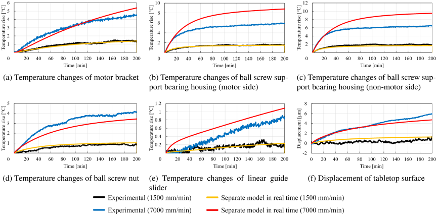
Fig. 9. Comparison of results from experiments and proposed approach at feed rates of 1500 mm/min and 7000 mm/min.
Regarding the results at 1500 mm/min, the temperature changes at each measurement point were in relatively good agreement. On the other hand, the thermal displacement itself was small, and the relative error was accordingly larger.
Regarding the results at 7000 mm/min, the temperature change of the nut was comparable to those observed under the other operating conditions. The temperature change of the linear guide slider showed a slight error. In the model used in this study, heat conduction between the linear guide slider and the guide rail is not considered. Since the heat generation at 7000 mm/min is greater than that under the other operating conditions and the resulting temperature change is also larger, it is possible that the temperature change is overestimated compared to the experimental results due to the neglect of heat conduction.
A significant error was observed in the temperature changes at the ball screw support bearing housings. The temperature changes were in good agreement up to approximately 15–20 min after the start of operation, where the temperature rose rapidly, and the error appeared thereafter. It is considered possible that the heat generation decreases as the temperature rises during operation. The ball screw in this apparatus is preloaded by pulling one end, thereby applying preload to the ball screw support bearings at both ends. In this state, the ball screw can be regarded as being axially supported at both ends. However, the preload tends to decrease due to thermal elongation of the ball screw shaft. In this experiment, the timing at which the preload would completely reach zero could be identified by observing the displacement at the shaft end during operation. Although the preload did not reach zero during operation, the displacement itself was larger compared to the other operating conditions, suggesting a possible influence on the heat generation behavior.
Therefore, the average motor current values during constant-speed movement were calculated from the servo data acquired during operation to examine how the current values changed over time. The results are shown in Fig. 10. As almost no difference was observed between the forward and return strokes, the current values of the forward stroke were adopted. Because the absolute current values differ depending on the conditions, the changes from the initial values are compared. Under all conditions, a decrease in the current values, i.e., a decrease in the torque required for operation, was observed from the start of operation. For the feed rates of 1500–5000 mm/min, the decrease was relatively small, whereas for 10000 mm/min and 7000 mm/min, a significant decrease over time was confirmed. At 7000 mm/min, a steep change was observed up to approximately 20 min from the start of operation, indicating that the resistance during table movement decreases. This is considered to be due to the reduction in axial preload caused by thermal elongation of the ball screw, as mentioned above. At 10000 mm/min, the change is smaller than that at 7000 mm/min, and the parameters for the heat generation estimation were identified using values that included this behavior; thus, relatively good agreement between the experimental and estimated results was confirmed.
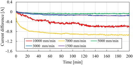
Fig. 10. Change in average motor current during constant-speed movement from the initial value under each feed rate condition.
On the other hand, even when the heat generation of the ball screw support bearings is not estimated with sufficient accuracy, the displacement at the tabletop surface is in reasonable agreement, indicating that the heat generation at the ball screw nut is the dominant factor.
For application to more general operating conditions, it is considered necessary to perform parameter identification over a wider range of conditions and to include factors such as the state change of the ball screw due to thermal elongation of the shaft in the model.
7. Conclusions
The authors have proposed methods to estimate, in real time, the temperature changes and displacements caused by the operation of a linear feed system. The performance of these methods has been verified by comparison with experimental results and the results of commercial FEM software. The conclusions obtained in this study are as follows:
-
1.
The parameters to estimate the heat generation values from the servo data were identified for the real-time estimation. Using these parameters and the servo data, the temperature changes were estimated with sufficient accuracy.
-
2.
By performing heat transfer analysis using the FVM, the temperature changes were successfully simulated in agreement with the experimental results. Furthermore, the results were compared with the commercial FEM software results, and good agreement was confirmed.
-
3.
With regard to the estimation of thermal dis-placement, we considered that using FEM for the whole model is unsuitable for rapid calculation; therefore, the linear estimation model and FEM of only the ball screw shaft and the table were employed, and a certain level of alignment with the experimental results was confirmed.
-
4.
Simulations were carried out using models in which the table and the bed were separated into individual models in order to cope with general operating conditions. Without considering the effects of heat conduction at the contact surfaces, such as the ball screw and the linear guides, the estimation accuracy was confirmed to deteriorate. Then, the heat conduction was simulated in a simplified manner based on the surface cell temperatures, and the estimation accuracy was improved.
-
5.
The proposed approach was evaluated by comparing the results with experiments under practical operating conditions. While the temperature changes and thermal displacements showed reasonable agreement in some aspects, a significant error was observed in the temperature changes at the ball screw support bearing housings. To apply the proposed approach to a wider range of operating conditions, it is necessary to perform parameter identification under more diverse conditions and to incorporate factors such as the change in the state of the ball screw due to thermal elongation of the shaft into the model.
- [1] S. Wakiya, R. Ishida, J. Kusuyama, and Y. Nakao, “Temperature control performance of a built-in motor spindle by developed temperature feedback control system,” Int. J. Automation Technol., Vol.17 No.5, pp. 512-520, 2023. https://doi.org/10.20965/ijat.2023.p0512
- [2] T. Liu, C. Li, Y. Zhang, W. Gao, Z. Fu, J. Zhang, and D. Zhang, “Active coolant control onto thermal behaviors of precision ball screw unit,” The Int. J. of Advanced Manufacturing Technology, Vol.119, pp. 1867-1882, 2022. https://doi.org/10.1007/s00170-021-08413-4
- [3] H. Shi, B. He, Y. Yue, C. Min, and X. Mei, “Cooling effect and temperature regulation of oil cooling system for ball screw feed drive system of precision machine tool,” Applied Thermal Engineering, Vol.161, Article No.114150, 2019. https://doi.org/10.1016/j.applthermaleng.2019.114150
- [4] K.-Y. Li, W.-J. Luo, X.-H. Hong, S.-J. Wei, and P.-H. Tsai, “Enhancement of machining accuracy utilizing varied cooling oil volume for machine tool spindle,” IEEE Access, Vol.8, pp. 28988-29003, 2020. https://doi.org/10.1109/ACCESS.2020.2972580
- [5] S. Zeng, J. Liu, and C. Ma, “Topology optimization in cooling moving heat sources for enhanced precision of machine tool feed drive systems,” Int. J. of Thermal Sciences, Vol.202, Article No.109065, 2024. https://doi.org/10.1016/j.ijthermalsci.2024.109065
- [6] C. Brecher and A. Wissmann, “Compensation of thermo-dependent machine tool deformations due to spindle load based on reduced modeling effort,” Int. J. Automation Technol., Vol.5 No.5, pp. 679-687, 2011. https://doi.org/10.20965/ijat.2011.p0679
- [7] Y. Sasaki, H. Iwai, Y. Wakazono, Y. Sakurai, and Y. Oka, “Development of real-time thermal displacement compensation system,” J. of the Japan Society for Precision Engineering, Vol.83, No.2, pp. 121-124, 2017 (in Japanese).
- [8] L. Weng, W. Gao, D. Zhang, T. Huang, G. Duan, T. Liu, Y. Zheng, and K. Shi, “Analytical modelling of transient thermal characteristics of precision machine tools and real-time active thermal control method,” Int. J. of Machine Tools & Manufacture, Vol.186, Article No.104003, 2023. https://doi.org/10.1016/j.ijmachtools.2023.104003
- [9] T.-J. Li, C.-Y. Zha, and Y.-M. Zhang, “Real-time thermal error prediction model for CNC lathes using a new one-dimension lumped capacity method,” The Int. J. of Advanced Manufacturing Technology, Vol.117, pp. 425-436, 2021. https://doi.org/10.1007/s00170-021-07692-1
- [10] A. Naumann, D. Ruprecht, and J. Wensch, “Toward transient finite element simulation of thermal deformation of machine tools in real-time,” Computational Mechanics, Vol.62, pp. 929-942, 2018. https://doi.org/10.1007/s00466-018-1540-6
- [11] T.-C. Chen, C.-J. Chang, J.-P. Hung, R.-M. Lee, and C.-C. Wang, “Real-time compensation for thermal errors of the milling machine,” Applied Sciences, Vol.6, No.4, Article No.101, 2016. https://doi.org/10.3390/app6040101
- [12] Y. Yang, J. Lv, Y. Xiao, X. Feng, and Z. Du, “Enhanced modeling method of thermal behaviors in machine tool motorized spindles based on the mixture of thermal mechanism and machine learning,” J. of Intelligent Manufacturing, Vol.36, pp. 221-242, 2025. https://doi.org/10.1007/s10845-023-02234-w
- [13] G. Chen and K.-C. Wang, “Real-time thermal error compensation of machine tools based on machine learning model and actual cutting measurement via temperature sensors,” Sensors and Materials, Vol.36, No.10, pp. 4221-4238, 2024. https://doi.org/10.18494/SAM5110
- [14] Z. Zhan, S. Wan, X. Li, and B. Fang, “Thermal behavior prediction of the spindle-bearing system based on the adaptive thermal network modeling method,” Engineering Applications of Artificial Intelligence, Vol.145, Article No.110199, 2025. https://doi.org/10.1016/j.engappai.2025.110199
- [15] P. Blaser, F. Pavlicek, K. Mori, J. Mayr, S. Weikert, and K. Wegener, “Adaptive learning control for thermal error compensation of 5-axis machine tools,” J. of Manufacturing Systems, Vol.44, pp.302-309, 2017. https://doi.org/10.1016/j.jmsy.2017.04.011
- [16] H. J. Pahk and S. W. Lee, “Thermal error measurement and real time compensation system for the CNC machine tools incorporating the spindle thermal error and the feed axis thermal error,” The Int. J. of Advanced Manufacturing Technology, Vol.20, pp.487-494, 2002. https://doi.org/10.1007/s001700200182
- [17] D.-H. Kim and J.-Y. Song, “Development of thermal deformation compensation device and CNC based real-time compensation for advanced manufacturing,” Int. J. of Automotive Technology, Vol.14, No.3, pp. 423-428, 2013. https://doi.org/10.1007/s12239-013-0046-7
- [18] M. Lei, F. Gao, Y. Li, P. Xia, L. Zhao, and J. Yang, “Feedback control of the mechanical spindle thermal error based on thermal simulation with bearing heat sources analysis,” J. Mechanical Engineering Science, Vol.238, No.1, pp. 249-263, 2024. https://doi.org/10.1177/09544062231171027
- [19] T. Tsutsumoto and K. Hasegawa, “Estimation of surface heat transfer coefficient by cooling of heated copper plate,” Bulletin of The Hiroshima Prefectural Technology Research Institute Western Region Industrial Research Center, No.63, Article No.10, 2020 (in Japanese).
- [20] R. Sato, M. Tsutsumi, and D. Imaki, “Experimental evaluation on the friction characteristics of linear ball guides,” Trans. of the Japan Society of Mechanical Engineers Series C, Vol.73, No.734, pp. 2811-2819, 2007 (in Japanese).
- [21] The Japan Society of Mechanical Engineers, “JSME Textbook Series Mechanics of Materials,” 2007 (in Japanese).
- [22] The Japan Society of Mechanical Engineers, “JSME Data Book: Heat Transfer 5th Edition,” 2009 (in Japanese).
- [23] Japan Society of Thermophysical Properties, “Thermophysical Properties Handbook,” 2008 (in Japanese).
This article is published under a Creative Commons Attribution-NoDerivatives 4.0 Internationa License.