
Research Paper:
Automated Dimensional Inspection of Knotted Nets Using YOLOv11 and K-Nearest Neighbors Regression
Muhammad Haziq Noor Akashah*,†
 , Masako Yamamoto**, and Naoki Uchiyama*
*Department of Mechanical Engineering, Toyohashi University of Technology
1-1 Hibarigaoka, Tempaku-cho, Toyohashi, Aichi 441-8580, Japan
†Corresponding author
**Amita Company
Toyohashi, Japan

Ensuring consistent mesh geometry is essential for mechanical reliability and quality control of knotted nets in factory production line inspections. This paper presents a fully automated visual inspection system that integrates knot detection, mesh topology reconstruction, and real-world dimensional measurements within a distortion-aware deep learning framework. The knots were detected using a YOLOv11-based object detector trained to localize small and densely arranged targets under varying illumination, deformation, and partial occlusion. To enable accurate metric measurements over large net areas, the images captured using a 150° ultrawide-angle lens were rectified through camera calibration and distortion correction. Knot centroids were extracted from the detected bounding boxes and organized using a row-wise directional linking strategy that reconstructed a diamond-shaped mesh topology while avoiding physically implausible connections. Interknot distances were computed in the rectified image plane and converted into real-world measurements using a K-nearest neighbors (KNN) regression model, which compensated for the residual nonlinearities remaining after distortion correction. The scope of inspection in this study was limited to mesh size and knot spacing evaluation. However, missing knots, broken strands, or other structural defects may affect the dimensional consistency of the net and may be indicated indirectly through abnormal mesh measurements. The proposed system is not intended for direct detection or classification of such defects. It was evaluated on a custom dataset of 1,054 industrial fishing net images, achieving a high detection performance with an mAP50 of 0.99 and mAP50–95 of 0.86. The calibration stage achieved distance estimation errors within ±3.53% relative to the nominal mesh size. The results demonstrated that the proposed approach enabled the automated and quantitative assessment of mesh uniformity, providing a practical and scalable solution for industrial net quality inspection.
1. Introduction
Net-based products play a critical role in fishing, agriculture, construction, packaging, and filtration industries because of their lightweight structure, flexibility, and mechanical robustness. The structural performance of nets fundamentally depends on the geometric integrity of the mesh, which is governed by the formation, positioning, and spacing of the knots 1. Even small deviations such as irregular mesh spacings, missing knots, or local distortions can significantly affect the load distribution and reduce the overall strength, ultimately leading to failure during use.
As industrial production volumes increase, maintaining consistency in knot formation is essential not only for mechanical reliability but also for operational safety and economic efficiency. Historically, net inspection has relied on manual visual approaches involving either skilled workers directly examining the mesh or in the context of aquaculture, professional divers or remotely operated vehicles (ROVs) performing underwater assessments 2. Although these methods can detect major abnormalities, they are highly labor-intensive, subjective, and inconsistent, particularly under varying lighting conditions, worker fatigue, and environmental disturbances. Manual inspection inherently lacks scalability. As modern production lines demand higher throughput and tighter quality control, the limitations of human-based inspection have become increasingly evident.
The need for reliable and automated inspections extends beyond manufacturing efficiency. In marine aquaculture, small defects such as ruptures, misaligned knots, or accidental openings can lead to large-scale fish escapes, causing ecological disturbances, spread of invasive species, and substantial financial losses 3,4. In agriculture and construction, defects in shade nets or safety nets compromise structural performance and increase operational risks. These scenarios underscore the importance of developing automated and accurate inspection systems that can detect subtle defects in net structures with minimal human intervention.
Although fishing net inspection is a specialized domain, similar challenges appear in the textile and yarn industries, where structural uniformity plays an equally critical role. Yarn evenness, which is defined as the uniformity of the fiber mass distribution along the length of the yarn, directly affects the fabric strength, dye consistency, and overall product appearance 5. Variations in yarn thickness or neps can lead to mechanical failure and visible defects, resulting in fabric rejection and financial losses 6,7. Classical inspection methods for yarn and fabrics such as filtering, thresholding, morphological operations, and edge detection 8,9,10,11 have been historically useful but are limited to real-world factory environments because of their sensitivity to lighting, texture variability, and noise. These illustrate the broader trend toward automated visual inspection systems capable of identifying small, repetitive structural units with high spatial precision.
Advances in machine learning and deep learning have dramatically improved the automated inspection of textiles and patterned materials. Convolutional neural networks (CNNs) have shown high accuracy in detecting defects in fabrics and woven structures by learning rich hierarchical feature representations directly from the data 12. Among deep learning architectures, the You Only Look Once (YOLO) family has emerged as a leading solution for industrial inspection applications, offering a strong balance between detection accuracy and inference speed 13. YOLO-based methods have been applied for the detection of fabric defects, yarn anomalies, and irregularities in mesh-like structures 14,15.
Despite the success of these methods, detecting small, densely packed knots in fishing nets remains challenging because of the limited pixel representation, repetitive structural patterns, occlusions, and varying lighting conditions. In this study, we proposed a framework that addressed these challenges using separate but connected modules. The limited pixel representation of the knots was addressed using a YOLOv11-based detector trained on high-resolution annotated images and resized inputs suitable for small object detection. Repetitive mesh patterns were handled after detection by converting the bounding boxes into centroids and applying a row-wise linking logic that used the expected diamond mesh structure. Occlusions and missed detections were mitigated by restricting candidate links to local neighboring rows and columns and omitting uncertain links, rather than forcing long-range connections. Variations in illumination and local net appearance were addressed through dataset diversity and data augmentation during training. Finally, geometric distortion and nonlinear pixel-to-distance scaling were addressed using wide-angle camera correction and K-nearest neighbors (KNN)-based calibration.
The latest YOLOv11 architecture introduces several enhancements, including multiscale feature fusion, anchor-free prediction, and adaptive label assignment 16. These improvements make YOLOv11 well suited for knot detection. However, existing studies on net inspection seldom integrate object detection with geometric measurements, mesh reconstruction, or real-world spacing analysis. Most previous studies are focused solely on defect classification rather than performing spatially precise measurements of the mesh geometry, which is essential for evaluating product quality.
Another major challenge in this domain is the use of ultrawide-angle lenses for industrial inspection. To increase the visual coverage of large net sections and reduce the number of viewpoints required, wide field-of-view cameras, including fisheye lenses, are commonly adopted, because a single image can capture a large portion of the scene 17,18. However, such lenses introduce substantial radial distortion, causing straight lines to bend and altering the geometric mapping between the pixel and real-world distances. Without distortion correction, equal pixel distances across the image do not correspond to equal physical distances, making precise measurements impossible. A few studies have directly addressed distortion correction in conjunction with deep-learning-based knot detection.
In this study, we addressed these critical gaps by proposing an automated knot inspection system that integrated YOLOv11-based detection, wide-angle camera distortion correction, directional linking logic for mesh reconstruction, and machine-learning-based real-world distance estimation. The system detected knots with high accuracy, reconstructed the mesh topology by linking adjacent knots, and computed real-world distances using a calibrated KNN regression model. Distortion correction ensured that spatial relationships were preserved even when using 150° ultrawide-angle lenses, enabling accurate measurements across the entire image plane.
The contributions of this study are threefold. First, we introduced a complete end-to-end pipeline for knot detection and mesh reconstruction using a modern YOLOv11-based detector capable of handling small and densely arranged targets. Second, we integrated camera correction and data-driven calibration to enable precise real-world distance measurements after detection, thereby bridging the gap between image-space processing and physical inspection. Third, we demonstrated a practical, scalable, and motion-triggered high-accuracy inspection solution suitable for industrial deployment, overcoming the limitations of classical image processing, and complementing previous work on textile and woven structure inspection.
Overall, we established a robust foundation for automated net quality evaluation by combining high-accuracy deep learning detection with geometric analysis and measurement capabilities, which are essential for modern industrial applications. The scope of this study was limited to factory-based production line inspection, where the camera was fixed beneath the net machine and imaging was performed in an indoor factory environment. Although fishing nets are also used in aquaculture and outdoor marine environments, we did not consider underwater imaging, water turbidity, surface reflection, hydrodynamic net deformation, or diver/ROV-based inspection in this study. Therefore, the proposed method should be interpreted as a production line dimensional inspection framework rather than a general underwater net inspection system.
2. Development and Evaluation of a YOLO-Based Detection System
The proposed YOLOv11-based inspection system was structured into several stages, each addressing a specific aspect of automated net quality assessment. An overview of the system configuration is presented in Fig. 1.
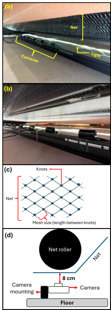
Fig. 1. (a) Camera placement located beneath the machine, (b) close-up image of the camera facing the net beneath the machine, (c) identification of the net components, and (d) side view of the camera facing the net in parallel.
2.1. Dataset Preparation and Wide-Angle Camera Distortion Correction
A custom dataset comprising 1,054 high-resolution images was collected from an industrial net production line. The images were originally captured at a resolution of \(1920 \times 1080\) pixels using a Sanwa Supply wide-lens webcam (USB connection, 150° ultra-wide-angle field of view, 2 megapixels, CMS-V53BK). During the image acquisition, the camera was fixed beneath the production machine at an approximate camera-to-net distance of 8 cm. The same camera position and imaging setup were used for both the dataset collection and production line testing. Although the images were resized to \(640 \times 640\) pixels for YOLOv11 inference, the knot size measurements were converted back to the original \(1920 \times 1080\) image scale. In the original image scale, individual knots were typically represented by approximately \(22 \times 12\) pixels, corresponding to an area of about 264 pixels\(^2\). Based on 146 sampled knots, the approximate knot size ranged from 13 pixels to 33 pixels in width and from 12 pixels to 30 pixels in height. This camera was selected because of its ability to capture large net sections with high spatial coverage, while maintaining sufficient image resolution. The captured images included multiple sections of the net observed under different orientations and perspectives, thereby increasing the dataset diversity while preserving adequate detail for accurate knot detection.
For model training, all images were resized to \(640 \times 640\) pixels to conform to the input requirements of YOLOv11, while balancing computational efficiency with sufficient feature representation. Resizing the original \(1920 \times 1080\) images to \(640 \times 640\) inevitably reduced the pixel representation of individual knots. However, the knots remained visible and detectable because their bounding boxes, when mapped back to the original image scale, were approximately \(22 \times 12\) pixels. The use of high-resolution source images also helped preserve sufficient knot texture and contrast after resizing. Cropping or tiling was considered as an alternative approach to preserve more local details for small knots. However, a full-frame \(640 \times 640\) input was selected in this study because it retained the global row-wise mesh arrangement required by the linking logic, avoided duplicate detections across tile boundaries, and simplified the inference process computationally. Cropping or tiling may be beneficial for future applications involving smaller knots, larger images, or more severe scale variations. To ensure accurate spatial measurements and preserve real-world distance relationships, all images captured with the 150° ultrawide-angle lens were preprocessed using a camera distortion correction procedure, as illustrated in Fig. 2.
The intrinsic camera parameters (\(f_x\), \(f_y\), \(c_x\), and \(c_y\)) and lens distortion coefficients (\(k_1\), \(k_2\), \(k_3\), \(p_1\), and \(p_2\)) were obtained using a standard camera calibration procedure based on a planar checkerboard pattern 19,20. Multiple images of a known checkerboard (a \(6 \times 8\) grid with a square size of 20 mm) were captured at different orientations and positions under uniform illumination.
The checkerboard corner points were automatically detected using OpenCV’s findChessboardCorners() function, and the camera parameters were estimated using the calibrateCamera() function. This process minimized the reprojection error between the observed and projected corner points, yielding an optimized camera matrix and distortion coefficients that characterized the lens geometry. The resulting parameters were then applied to image rectification using cv2.undistort() prior to model training.
The distortion correction followed the standard pinhole camera model combined with the Brown–Conrady radial-tangential distortion formulation.
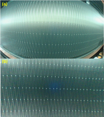
Fig. 2. (a) Original image captured using a 150° ultrawide-angle lens and (b) rectified image after distortion correction.
The intrinsic camera matrix \(K\) is defined as
The radial and tangential distortions are modeled as
The dataset reflects a broad range of real-world conditions, including varying lighting environments and zoomed-in and zoomed-out views 21. All images were meticulously annotated with bounding boxes using Roboflow, which provides a user-friendly annotation interface, consistent labeling formats, and integrated quality control tools.
This ensured precise and standardized ground-truth labels for supervised training, while also facilitating dataset versioning and direct export in formats compatible with YOLOv11. To promote robust generalization of unseen production scenarios, the dataset included realistic variations in knot orientation, mesh scale, deformation, and illumination. The dataset was divided into training, validation, and testing subsets using a 70%–15%–15% split, ensuring representative distributions of net configurations across all subsets.
The 100 randomly selected fishing net images described in Section 4.2 were collected separately during production line testing while the machine was running. These images were captured using the same camera setup as the training, validation, and testing datasets, but they were used as an additional practical evaluation set to assess the detection and linking performance under operating conditions. Sample images from the dataset, illustrating the variations in the imaging conditions, are shown in Fig. 3.
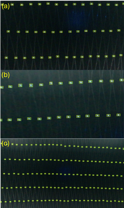
Fig. 3. Sample images from the net dataset showing different imaging conditions: (a) low-light image, (b) zoomed-in image with a smaller visible net region, and (c) zoomed-out image with a wider field of view and more visible knot rows.
2.2. Model Selection and Training
The YOLOv11m (medium) variant was selected as the detection backbone to balance the detection accuracy and computational efficiency, making it suitable for deployment on production hardware. Larger variants such as YOLOv11L and YOLOv11XL generally achieve higher mean average precision (mAP); however, their increased parameter counts and computational demands significantly reduce the inference speed. This trade-off makes them less appropriate for continuous, high-throughput inspection tasks.
Given that the primary system requirement was reliable knot detection under triggered or intermittent high-accuracy inspection, YOLOv11m was selected as an effective compromise between precision and processing speed. The YOLOv11m model contains approximately 13.8 million parameters and requires 28 giga floating point operations per second (GFLOPs) per inference. Compared with the lightweight YOLOv11n variant, it offers higher detection precision while maintaining a practical inference speed for downstream tasks such as distance estimation and defect classification. This balance ensures a smooth integration into the inspection workflow with manageable graphics processing unit (GPU) requirements and acceptable latency.
Training was performed on a custom-annotated dataset using transfer learning from pretrained YOLOv11m weights. The model was trained for 200 epochs with a batch size of 16 and input resolution of \(640 \times 640\) pixels. Automatic mixed precision (AMP) was used to accelerate training and reduce GPU memory consumption. To improve generalization and robustness, a range of data augmentation techniques were applied, including random scaling, translation, brightness variation, horizontal flipping, mosaic augmentation (disabled after the first 10 epochs), copy–paste augmentation, and random erasing. These augmentations enhanced the robustness to variations in net geometry, orientation, and illumination conditions.
By leveraging the improved accuracy of the YOLOv11m variant and comprehensive data augmentation, the trained system achieved high-precision knot detection while maintaining acceptable latency for triggered inspection. This made the proposed approach well-suited for deployment in industrial-scale inspection environments without compromising detection reliability.
2.3. Assessment of the Detection Model
The trained knot detection model was assessed using established object detection metrics: precision (\(P\)), recall (\(R\)), and mean average precision (mAP). Evaluations were performed both at a fixed intersection-over-union (IoU) threshold of 0.5 and across a range of thresholds from 0.5 to 0.95. The precision measures the fraction of correct detections among all predictions, whereas the recall expresses the fraction of correctly identified knots relative to the total number of ground-truth instances. The formal definitions of these metrics are given in Eqs. (5) and (6), following 22.
In this study, \(c = 1\), because the model was trained specifically to identify knots in the fishing nets. During training, the loss components associated with the bounding box regression, classification, and objectness were tracked. As illustrated in Fig. 4, these loss values decreased steadily and converged after approximately 180 epochs, suggesting that the network successfully captured the relevant visual features for knot detection.
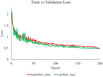
Fig. 4. Training and validation loss curves across 200 epochs.
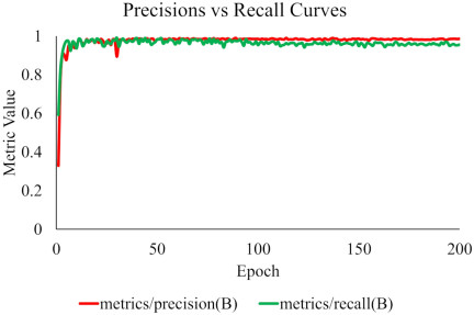
Fig. 5. Precision and recall curves obtained on the validation set during YOLOv11 training.
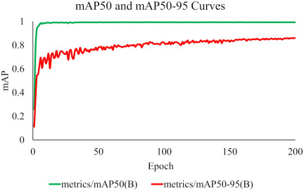
Fig. 6. Validation set average precision curves reported in terms of mAP50 and mAP50–95.
The curves shown in Figs. 5 and 6 correspond to validation set performance during YOLOv11 training and evaluation. They were generated using the validation subset defined in Section 2.1 and were separated from the additional 100-image production line evaluation described in Section 4.2. The progression of precision and recall values, shown in Fig. 5, indicated that both metrics stabilized after approximately 50 epochs. Their high values, approaching 100%, confirm the robustness of the model when applied to diverse net images.
Figure 6 shows the AP scores across the IoU thresholds. The model achieved nearly perfect detection, as indicated by the mAP50, as well as strong performance, as indicated by the mAP50–95 of 0.86, confirming robustness even under stricter evaluation criteria. The final trained detector achieved an overall accuracy of 0.983 and a recall of 0.979, indicating that 98.3% of the predictions were correct and 97.9% of all knots were successfully localized. These results highlight the effective balance between precision and recall, thereby reinforcing the suitability of the model for deployment on automated net inspection systems.
In conclusion, the YOLOv11m-based detector demonstrated high reliability in identifying knots under different conditions of overlap and deformation. Its high detection accuracy and efficiency render it suitable for integration into real-world industrial inspection pipelines.
3. Inference Process and Knot Detection
During inspection, the trained YOLOv11 model predicted the bounding boxes and corresponding confidence scores for knot instances in each input frame. The confidence threshold was set to 0.05. This relatively low threshold was selected to prioritize recall because the knots were small objects and missed detections could interrupt the subsequent linking process 23. Potential low-confidence false positives were further filtered indirectly by the row-wise linking logic, which only accepted geometrically plausible neighboring knots. Consequently, only reliable knot candidates were retained for subsequent processing and analysis.
The inference performance of the proposed system was evaluated using single-image forward passes. On the test platform, the model achieved an average inference time of approximately 1230 ms per image, corresponding to an inference speed of 0.81 frames per second (fps). The intended operational scenario was a motion-triggered production line inspection rather than a continuous frame-by-frame video analysis. In the implemented system, the camera continuously streamed the calibrated frames, and a motion-trigger module compared the consecutive grayscale frames using Farneback optical flow. The average optical flow magnitude was calculated, and when it exceeded a preset threshold of 0.5, the system interpreted this as the movement of the net between frames and captured the current calibrated frame for prediction. Therefore, the production line did not need to stop for each inspection; rather, the system sampled the newly presented net regions when motion was detected.
Accordingly, the reported speed of 0.81 fps should be interpreted as the processing speed for each triggered inspection image, not as the frame rate of continuous video inspection. The current implementation was suitable for triggered or intermittent inspections, where the interval between inspection events was compatible with a processing time of approximately 1230 ms. Although the current implementation prioritized detection accuracy over computational speed, further optimization, such as model compression or hardware acceleration, can be explored to improve the real-time capability in future deployments.
3.1. Knot Position and Centroid Extraction
Once the YOLOv11 model detects a knot, it is localized by a bounding box, which is defined as
These centroids provide a precise spatial representation of the knot positions within the image. Formally, the set of all the knot centroids is denoted as
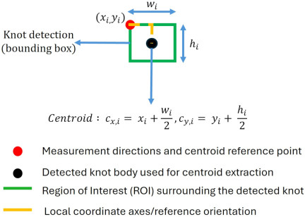
Fig. 7. Knot detection and centroid extraction.
3.2. Linking Logic and Distance Measurement Using KNN Regression Model
The KNN regression model was selected because the pixel-to-distance relationship after wide-angle correction was not strictly linear across the image plane. Although camera undistortion reduced the dominant radial distortion, residual nonlinear effects could still persist because of the ultrawide lens, local perspective variation, centroid localization error, and small changes in the knot shape. A global linear regression model represents the entire calibration range using a single slope and intercept, which may be insufficient in the presence of local variations. In contrast, KNN regression is a nonparametric local estimation method. For each measured pixel distance, the prediction is calculated from nearby calibration samples, rather than from a single global function. This makes the KNN regression model suitable for the proposed calibration task because the calibration samples cover the expected measurement range of the net, allowing local interpolation within the operating range. However, the KNN regression model is not intended for reliable extrapolation outside the calibrated range, and additional calibration points are required if the camera position, mesh size, or measurement region changes significantly.
The proposed linking logic was designed for regular knotted nets with a diamond-shaped mesh topology. In this topology, knots were arranged in staggered rows, and each knot was expected to connect diagonally to at most two neighboring knots in the next row. Therefore, this method assumed a repeated diamond mesh pattern, a fixed camera position, and a known target mesh eye size for calibration and quality assessment.
In practice, the row and column relationships are determined from the detected knot centroids. After knot detection, each bounding box was converted into a centroid coordinate \((c_{x}, c_{y})\). The expected mesh spacing in the pixels was estimated from the calibration model and target mesh size. The image height was then divided into row regions according to this expected spacing, whereas the image width was divided into column regions. Each detected centroid was assigned to a row and column index based on its pixel location.
For the centroid located in row \(r\) and column \(c\), the next row is defined as row \(r+1\). The same column refers to column \(c\) in the next row, while the adjacent columns refer to columns \(c-1\) and \(c+1\), when they exist. Therefore, the candidate knots for linking were searched only in row \(r+1\) and within columns \(c-1\), \(c\), and \(c+1\). This restricted search prevented long-range or physically implausible connections.
The linking logic connected knots sequentially from the top row to the bottom row to reconstruct the diamond-shaped mesh structure.
To illustrate this concept, one knot was selected as the reference knot and labeled \(K_0\), as shown in Fig. 8. Linking was performed only between two consecutive rows to avoid physically implausible long-range connections. For the reference knot \(K_0\), the candidate knots were searched exclusively in the immediately following row \((r+1)\) and restricted to the same column and its adjacent columns. This constrained search region ensured that only local and physically valid neighbors were considered.
The candidate knots were then divided into two groups according to their horizontal positions relative to \(K_0\). The knots located to the left of \(K_0\) formed the left candidate set \(C_L\), and the knots located to the right formed the right candidate set \(C_R\). The nearest knot was selected from each candidate set to form the diagonal connections. The closest knot in \(C_L\) was labeled \(P_L\), and the closest knot in \(C_R\) was labeled \(P_R\), where the closeness was determined by the smallest horizontal displacement. If no candidate existed on one side, the corresponding connection was omitted. For each reference knot, the Euclidean distance to all candidate knots in the permitted neighboring cells was calculated. The candidates were sorted by distance, and up to two closest candidates were selected as links. This corresponded to the physical structure of a diamond-shaped knotted mesh in which each knot was connected diagonally to at most two knots in the next row. If no valid candidate was found on one side, that link was omitted rather than replaced by a distant knot.
Consequently, each knot established up to two diagonal links to the next row: a left link to the \(P_L\) and a right link to the \(P_R\). The same linking procedure was then applied to \(P_L\) and \(P_R\) as new reference knots in subsequent rows. Repeating this process row by row naturally produced the characteristic X-shaped and diamond-shaped mesh topologies observed in fishing nets.
For other net structures such as rectangular, square, hexagonal, or irregular mesh patterns, the knot detection stage can still be used if the knots are visually similar to those in the training data. However, the row-indexing strategy, neighbor-search region, expected number of links per knot, and quality threshold definition should be modified according to the corresponding mesh topology. In addition, the pixel-to-distance calibration should be repeated whenever the camera position, net type, or target mesh size changes.
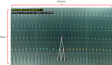
Fig. 8. Knot linking strategy. Each knot in a given row was connected to selected candidates in the subsequent row to form the diamond-shaped mesh pattern.
For each valid connection, the Euclidean distance is computed in pixel units and is defined as
The fishing net evaluated in this study was designed with the target mesh eye size \(\mu\), specified by the manufacturer as 100% (normalized measurement). This value represents the target reference against which all measured knot distances were evaluated. To avoid the disclosure of absolute dimensional specifications and enable a scale-independent evaluation, all the measured distances were normalized with respect to the target mesh size. The accurate conversion of pixel distances to real-world metric measurements is essential for quantitative quality assessment. Although a preliminary wide-angle correction was applied (Section 2.1), residual nonlinearities may persist in the rectified image plane because of the 150° ultrawide lens. The KNN regression model was selected as the candidate calibration model because it demonstrated strong performance in mapping pixel-based measurements to real-world targets in related visual inspection and net mesh size measurement tasks using YOLO-derived outputs 24,25. To address this issue, two regression approaches were evaluated using a calibration dataset comprising 45 distance measurements, as shown in Fig. 9.
Linear regression (LR) assumes global linear mapping, whereas KNN regression directly predicts the real-world distances based on local neighborhoods in the calibration data. The linear regression model is represented as
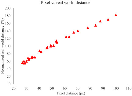
Fig. 9. Manually obtained real-world distance versus pixel distance used for calibration.
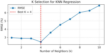
Fig. 10. K-selection curve for KNN regression. The optimal value \(k = 4\) minimized the RMSE on the testing set.
The dataset was divided into training and testing sets (80% and 20%, respectively) using stratified sampling to ensure representative coverage across the entire distance range. Hyperparameter optimization for the KNN regression model was performed for \(k = 1\)–10, and the model performance was evaluated on the held-out testing set using the root mean square error (RMSE), mean absolute error (MAE), and coefficient of determination \(R^2\) metrics. As shown in Fig. 10, the optimal value was \(k = 4\), which yielded the smallest prediction error. Using the testing set, the KNN regression model with \(k = 4\) achieved an MAE of 2.31%, RMSE of 2.45%, and \(R^2\) of 0.995, significantly outperforming the linear regression model (\(\textrm{MAE} = 3.94{\%}\), \(\textrm{RMSE} = 4.53{\%}\), and \(R^{2} = 0.983\)). These results indicated the presence of mild nonlinearities in the pixel-to-distance relationship, which the KNN regression model captured more effectively than the global linear regression model.
Figure 11 compares the predicted and actual distances for both regression models. The linear regression model exhibited systematic overestimation and underestimation, particularly at larger pixel distances, whereas the KNN regression model with \(k = 4\) closely followed the nonlinear calibration curve and significantly reduced the prediction error.
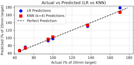
Fig. 11. Comparison of the predicted versus actual distances between the linear regression and KNN regression models.
Table 1 summarizes the numerical prediction results obtained for the representative test samples. The linear regression model showed consistent systematic bias across the calibration range, whereas the KNN regression model maintained substantially lower absolute errors, with all deviations confined to within \(\pm\)3.53%.
| Prediction [%] | Error [%] | ||||
| Pixel [px] | Actual [%] | LR | KNN | LR | KNN |
| 385.0 | 65.0 | 67.34 | 66.63 | +2.34 | +1.63 |
| 189.0 | 71.0 | 76.02 | 73.45 | +5.02 | +2.45 |
| 274.9 | 95.0 | 92.58 | 96.04 | -2.42 | +1.04 |
| 188.0 | 95.0 | 93.02 | 96.74 | -1.98 | +1.74 |
| 130.1 | 100.0 | 98.21 | 102.52 | -1.79 | +2.52 |
| 150.0 | 136.5 | 130.47 | 133.26 | -6.03 | -3.24 |
| 200.9 | 170.5 | 178.47 | 166.97 | +7.97 | -3.53 |
Each measured distance was evaluated against quality thresholds defined by \(\mu \pm \varepsilon\), where \(\mu\) denotes the expected mesh eye size and \(\varepsilon\) represents the user-defined tolerance. Connections were classified as acceptable, overtensioned, or undertensioned and were visualized using green, red, and orange lines, respectively. By enforcing directional, row-wise linking with constrained spatial neighborhoods, the proposed method preserved the mesh topology while enabling a reliable and interpretable quality assessment.
4. Results
4.1. Knot Detection
For evaluation, an \(\textrm{IoU} = 0.5\) was used as the main detection-matching threshold because it is a standard criterion for object-detection evaluation, following the PASCAL VOC evaluation protocol 26. In addition, mAP50–95 has been reported to provide a stricter assessment of the localization performance across multiple IoU thresholds, following the MS COCO evaluation protocol 27. The proposed YOLOv11-based detection framework demonstrated high accuracy in identifying knots within the fishing net images. For each detected knot, the model outputted a bounding box, parameterized by its top-left and bottom-right coordinates, as defined in Eq. (9). These bounding boxes provided not only the location but also the scale of each detected knot, ensuring robust detection even under varying lighting and background conditions.
From each bounding box, the centroid was calculated using Eq. (10) and served as a compact and representative feature of the spatial position of the knot. These centroids were particularly important because they formed the basis for distance calculations between knots, enabling the quantitative evaluation of mesh uniformity. Therefore, accurate centroid localization was a crucial step in the transition from object detection to geometric analysis of the net structure.
Figure 12 shows the sample outputs from the detection pipeline. The bounding boxes (green rectangles) delineate the detected knots and the corresponding centroids are marked by red points. This combination of bounding box detection and centroid extraction created a reliable representation of knot locations across the image, facilitating further processing stages, such as distance measurement, mesh consistency evaluation, and defect identification.
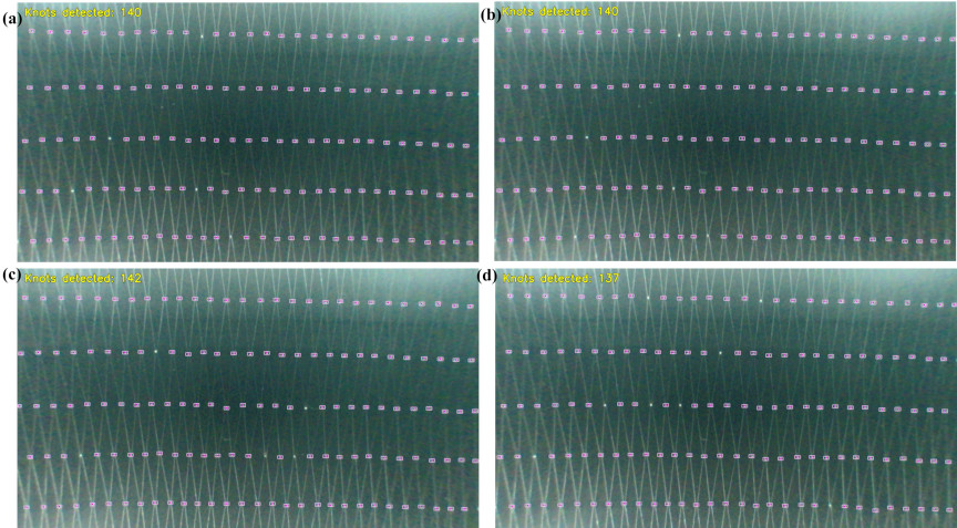
Fig. 12. Knot detection and centroid extraction. Bounding boxes represent YOLOv11 detections (magenta), whereas the dots indicate the computed centroids (magenta). Each image demonstrated a detected knot count of (a) 140, (b) 140, (c) 142, and (d) 137.
4.2. Detection Accuracy
To evaluate the knot detection performance, the proposed YOLOv11 model was tested on 100 randomly selected fishing net images. The ground-truth knot count (gt_count), detected knot count (det_count), and matched knot count (matched_count) were recorded for each image. The detection accuracy, computed as the ratio of matched predictions to ground-truth knots, ranged from 90.60% to 97.30%, with a mean value of 94.87%. These results show that the detector consistently localized most knots despite variations in lighting, contrast, mesh deformation, and partial occlusion. The results are summarized in Table 2.
Figure 13 shows the per-image accuracy distribution. The values clustered tightly at approximately 95%, demonstrating stable performance across diverse environmental and imaging conditions. Although the detector did not achieve a perfect score of 100%, this did not hinder the subsequent measurement stages. The linking logic relied on pairs of correctly detected knots and not on the exhaustive detection of every knot in the frame. Missed detection typically occurred near the image boundaries or in low-contrast zones that had a minimal contribution to the core measurement region. Thus, the mesh structure could still be reliably reconstructed.
| Metric | Value |
| Minimum detection accuracy | 90.60% |
| Mean detection accuracy | 94.87% |
| Maximum detection accuracy | 97.30% |
| Images above 95% accuracy | 31% |
| Images above 93% accuracy | 82% |
Furthermore, the YOLOv11 model achieved strong localization quality (\(\textrm{mAP50} = 0.99\) and \(\textrm{mAP50–95} = 0.86\)), indicating that nearly all detected knots had accurate bounding boxes. The small number of unmatched cases typically arose from annotation ambiguity or borderline detections, rather than systematic model failures. Because the downstream pipeline used the centroid positions of the correctly detected knots, the effect of these minor discrepancies on the real-world distance estimation was negligible. Overall, the achieved mean accuracy of 94.87% was sufficient to support the measurements of the proposed inspection system. The robustness of the detection stage provided a strong foundation for linking logic and geometric reconstruction, as described in the following section.
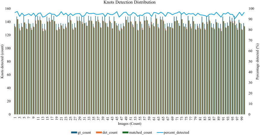
Fig. 13. Distribution of knot detection accuracy across 100 evaluation images.
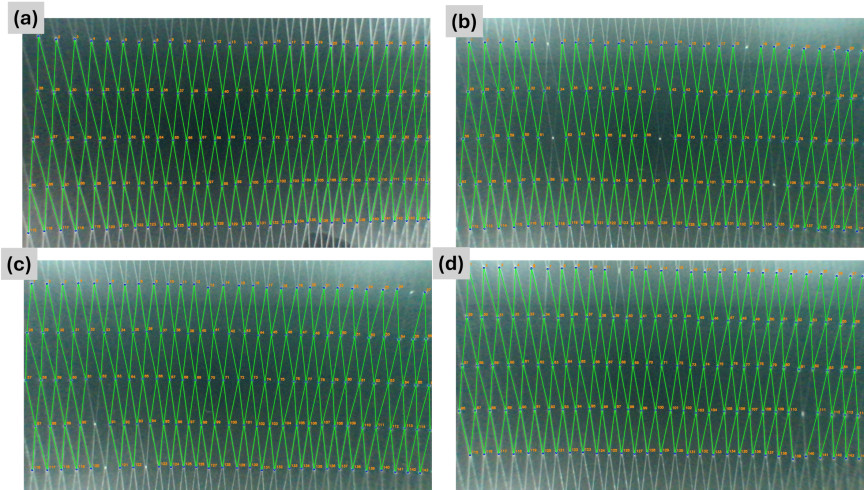
Fig. 14. Output of the linking logic showing the reconstructed X-pattern connections across the net with (a) a fully connected mesh and (b), (c) and (d) diverse scenarios of a partially connected mesh with some missing links due to undetected knots.
4.3. Linking Logic and Distance Measurement
Figure 14 shows the output of the proposed linking algorithm applied to the detected knot centroids. The reconstructed X-pattern accurately represented the geometric structure of the fishing net, demonstrating that the system could reliably group knots into aligned rows and form consistent diagonal and vertical connections. This behavior remained stable even in the presence of mild occlusion, irregular illumination, or small detection gaps. To quantitatively evaluate the robustness of this linking stage, a link success analysis was performed on 100 randomly selected evaluation images. The expected number of links was computed from the ground-truth annotations, whereas the predicted links were obtained from the linking logic based on the detected knots. The link success rate is defined as
| Metric | Minimum | Mean | Maximum |
| Detection accuracy [%] | 90.60 | 94.60 | 97.30 |
| Expected links | 250 | 264.3 | 279 |
| Predicted links | 211.5 | 237.9 | 256.5 |
| Link success [%] | 82.09 | 89.80 | 94.67 |
More importantly, the linking logic did not generate crossed, duplicated, or structurally inconsistent connections, even when knot detections were missing. Instead, it only omitted links for which insufficient evidence was available. Consequently, the reconstructed mesh remained geometrically valid and suitable for the subsequent pixel-to-millimeter conversion and quality assessment. This robustness ensured that the overall inspection pipeline functioned reliably under real-world production conditions, even when the detection stage was not flawless.
4.4. Real-World Distance Estimation
This methodology allowed the automated and quantitative measurement of fishing net mesh size, bridging the gap between image-based detection and actual net geometry. By leveraging the previously established linking logic, the system ensured that the measurements were derived from valid knot pairs, maintaining structural consistency while providing accurate real-world distance estimates.
An important factor influencing the measurement accuracy was the image rectification applied to compensate for the 150° ultrawide-angle lens. Although the undistortion step corrected most of the radial deformation, small residual nonlinearities persisted across the rectified image plane, particularly toward the periphery, where the stretching and compression effects were more pronounced. These residual distortions directly affected pixel-to-millimeter mapping, where equal pixel distances in different regions of an image did not always correspond to equal real-world distances. This necessitated the use of a data-driven regression model, particularly KNN regression, which adapted locally to the calibration data and compensated for the remaining nonlinear behavior more effectively than a global linear model.
To validate the reliability of the regression-based pixel-to-millimeter conversion, a comprehensive analysis was performed using 100 random samples collected within the expected ideal range. The KNN regression model generated the corresponding predicted measurements for each sample.
Figure 15 shows the three key diagnostic plots used to assess the model behavior. Fig. 15(a) shows the distribution of actual versus predicted mesh distances. Dense clustering along the one-to-one reference line indicated a strong agreement between the true and estimated values. Fig. 15(b) shows the prediction error distribution, which was sharply centered at zero, confirming the absence of systematic overestimation or underestimation. Finally, the residual distribution in Fig. 15(c) exhibited a scattered residual concentrating around zero, demonstrating stable model behavior and consistent generalization across the full range of measurements.
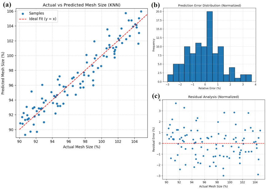
Fig. 15. Diagnostic plots for KNN regression performance: (a) actual versus predicted distances, (b) prediction error distribution, and (c) residual distribution.
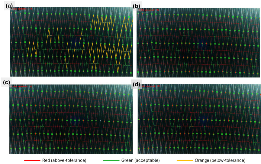
Fig. 16. Visualized quality classification of the fishing net based on real-world distance estimation. Colors indicate acceptable (green), below-tolerance (orange), and above-tolerance (red) mesh sizes. (a) shows the complete variations of the three colored lines whereas (b), (c), and (d) show only the red and orange colored lines.
In addition to these regression diagnostics, Fig. 16 provides a qualitative visualization of the final mesh measurement pipeline. The detected knot pairs were connected by color-coded lines, indicating the mesh size quality relative to the nominal specification. The reference mesh eye size of the evaluated fishing nets was considered to be 100%. In this study, the \(\pm\)5% tolerance band was selected arbitrarily for demonstration purposes and does not represent an industry standard or manufacturer-specified acceptance criterion. In practical deployment, the threshold should be replaced by the manufacturer’s specifications or an applicable quality control standard. The threshold was used only to illustrate how the proposed system could classify and visualize the mesh size deviations once a tolerance value was specified.
The KNN regression model showed a maximum observed prediction error of \(\pm\)3.53% for the test samples. Because this error was relatively close to the demonstration threshold of \(\pm\)5%, measurements near the decision boundary may be misclassified if evaluated from a single measurement alone. Therefore, the color-coded classification should be interpreted as a proof-of-concept visualization, rather than as a finalized industrial pass or fail rule.
In practice, borderline measurements should be performed using repeated measurements, a wider warning zone, or confirmation from neighboring mesh measurements.
Green lines represent measurements that fall within this tolerance range and therefore correspond to meshes that satisfy the nominal production requirement.
Orange lines indicate slightly undersized meshes, where the measured distance is less than 5% of the target mesh size, signaling localized compression or reduced tension. Red lines highlight oversized or overtensioned meshes in which the measured spacing exceeds 5% of the target mesh. These deviations may arise from manufacturing inconsistencies, uneven stretching, or local distortions during handling.
It is worth noting that for the purpose of demonstrating the sensitivity of the proposed inspection system, the net machine settings were intentionally left in a mildly nonoptimal configuration during this test. This setup introduced controlled variability in the mesh spacing, enabling the system to reveal a higher occurrence of orange and red classifications in the visualization. Consequently, Fig. 16 highlights the ability of the system to detect subtle deviations that may not be easily observed through manual inspection. The visualization illustrates not only the geometric reconstruction of the mesh but also the spatial distribution of quality deviations across the net. By encoding the measurement errors directly on the image, the system enabled the rapid identification of tension imbalances, gradual drift in mesh spacing, and localized defects that may require corrective action during production.
5. Discussion
The results of this study demonstrated that the proposed YOLOv11-based inspection system provided reliable and accurate knot detection for industrial net production. High-resolution image acquisition, meticulous annotation, and comprehensive model training enabled the system to capture fine-grained features of knots under diverse orientations, lighting conditions, and mesh deformations. A key contribution of this study is the application of camera correction to images captured using a 150° ultrawide-angle lens. The rectilinear transformation removed the wide-angle distortion, ensuring that the spatial relationships between knots were accurately represented. This preprocessing step was critical for reliable real-world distance estimation, as it allowed precise centroid localization and enhanced the robustness of the linking logic and Euclidean distance calculations. Camera correction directly improved the measurement fidelity and detection consistency, particularly near the peripheries of the images, where distortion would otherwise be most pronounced. The calibration dataset used for the pixel-to-millimeter conversion consisted of 45 manually measured distance samples selected to cover the pixel distance range observed in the production line images. The exact image plane coordinates of these calibration pairs were not recorded during the original measurement process, and therefore, the calibration model was evaluated primarily with respect to the sampled pixel distance range rather than a full two-dimensional spatial coverage map. Because the KNN regression model is a local interpolation method, a reliable prediction is expected only within the calibrated distance range and under the same camera setup used for the calibration. The model should not be interpreted as providing a reliable extrapolation to uncalibrated image regions, particularly near the image periphery, where the residual distortion after wide-angle correction may be more significant. If future deployment requires measurements across a wider field of view or near peripheral regions, additional calibration samples with recorded image coordinates should be collected and the regression model should be updated. This limitation is consistent with the nearest-neighbor nonparametric regression, where predictions are estimated from nearby calibration samples rather than from a global parametric function 28. Therefore, KNN regression is most appropriate for interpolation within the sampled calibration range and should not be treated as a reliable extrapolation method outside the calibrated data distribution. This consideration is particularly important for wide-angle imaging systems because camera calibration and residual distortion are influenced by the geometric distribution of the calibration observations across the image plane 19.
The importance of precise wide-angle calibration and distortion correction was highlighted in a previous study 29, in which improved automatic checkerboard detection and a Taylor-series-based mathematical model were proposed to calibrate both the intrinsic and extrinsic parameters of wide-angle cameras. The approach adopted in 29 demonstrated that an accurate radial distortion correction enabled reliable geometric measurements, supporting the rationale for our preprocessing pipeline.
For practical production line deployment, camera calibration was performed before installation, rather than beneath the operating net machine. The checkerboard images were captured in a controlled setup prior to mounting the camera, and the resulting intrinsic parameters and distortion coefficients were then stored and applied during operation. Because the same camera model and lens configuration were used across the inspection setup, the calibration parameters could be applied consistently to other cameras with the same optical configuration, provided that their resolution and lens setting remained unchanged. During operation, it was not necessary to insert a checkerboard beneath the machine. Instead, the calibration validity should be verified periodically using a reference image or a reference net captured under a normal camera setup. Recalibration should be performed if the camera is replaced, or when there are changes in the lens settings, image resolution, or mounting position. The drift caused by machine vibrations was expected to be minimal because the camera setup was installed separately from the production machine and did not contact its components. The remaining practical factors, such as lens contamination or temperature-related optical changes, could be monitored through periodic reference checks and routine lens inspections.
The trained YOLOv11m model achieved an mAP50 of nearly 1.0 and mAP50–95 of 0.86, indicating high detection precision, even under challenging conditions. Accurate centroid extraction enabled the organization of knots into mesh-aligned rows and the construction of an X-pattern linking logic, facilitating the automated quantification of knot spacing and mesh uniformity. The machine-learning-based calibration model successfully converted pixel distances into real-world measurements, validating the ability of the pipeline to bridge image-based detection and physical net geometry.
The calibration experiment further highlights the importance of selecting a regression model that can accommodate residual nonlinearities after wide-angle distortion correction. Although the LR model provided a simple global fit, its RMSE of 4.53% indicated that it could not fully represent the subtle nonlinear mapping between the pixel distance and physical millimeter spacing. In contrast, the KNN regression model with \(k = 4\) reduced the RMSE to 2.45% and achieved a higher \(R^2\) of 0.995. This improvement is attributed to the locality-based interpolation of the KNN regression model, which captures fine variations in the calibration data arising from the lens characteristics, knot shape, and centroid extraction noise. These findings confirmed that KNN was better suited for high-precision measurement tasks using the proposed inspection system.
In the broader context of textile and mesh inspection, fabric quality plays a crucial role in modern industrial processes, and the rapid and effective detection of defects is a primary research goal. Previous studies highlighted the challenges of detecting small-scale objects in complex structures. For example, 30 proposed an improved YOLOv4-based approach for detecting tiny fabric defects by integrating advanced data augmentation, \(k\)-means-based anchor clustering, additional prediction layers, attention modules, and a modified loss function (CEIOU). This resulted in a 12% increase in the AP for tiny targets and a 3% overall improvement in the mAP, demonstrating that combining model architectural improvements with targeted preprocessing could substantially enhance detection performance.
In this study, we addressed the challenges of small and densely arranged objects (knots) by leveraging the multiscale feature fusion and anchor-free detection of YOLOv11 combined with camera correction and calibration for accurate spatial measurements. Compared with traditional blob detection or classical image processing approaches, the proposed deep learning system exhibited superior robustness to variations in lighting, deformation, and object density.
An earlier study 31 used a multichannel blob detection algorithm based on real Gabor functions for texture segmentation during textile inspection. The method extracted texture features across multiple orientations and spatial frequencies, where the real part of the Gabor function acted as a blob detector sensitive to local contrast and structural irregularities. Through multichannel filtering and nonlinear local energy estimation, the defects were segmented by differentiating abnormal texture responses from normal fabric patterns.
Although this approach achieved high accuracy for periodic textile structures and offered computational efficiency suitable for real-time inspection, its performance depended heavily on filter tuning, fixed illumination, and handcrafted thresholds for sensitivity control.
In contrast, our YOLOv11-based inspection system benefited from deep feature extraction and end-to-end optimization and automatically learned discriminative spatial and contextual representations from training data without manual feature engineering. As reported in 32, the YOLO11 architecture and its adaptive variants (such as AED-YOLO11) leverage frequency-domain aggregation, efficient attention compression, and dynamic upsampling to enhance small object detection and spatial accuracy. These architectural improvements enable the robust recognition of fine-scale targets even under noise, deformation, and low-contrast conditions, which are scenarios in which blob-based or filter-driven algorithms typically degrade. The frequency-spatial fusion and adaptive channel-weighting mechanisms in the backbone and neck modules of YOLOv11 allow context-aware feature extraction across multiple resolutions, leading to improved generalization and precision in complex inspection environments. Consequently, our YOLOv11-based inspection system demonstrated superior adaptability for detecting small, densely arranged knots while maintaining computational efficiency, highlighting the advantages of data-driven deep learning frameworks over traditional blob detection in modern visual inspection tasks.
However, several limitations remain in this study. For example, the dataset of 1,054 images may not fully encompass all net types, materials, or production scenarios. Our YOLOv11-based inspection system also assumes a fixed camera distance, and deviations from this distance can introduce perspective errors unless additional calibration is applied.
Furthermore, deployment on resource-constrained edge devices may require lightweight architectures or model compression. The findings of this study can serve as a basis for extending the dataset to improve generalization, integrating multiple camera views or performing 3D reconstruction for a more comprehensive spatial analysis, exploring lightweight hybrid models for edge deployment 33, and incorporating automatic defect classification with real-time corrective feedback.
Overall, the proposed system demonstrated the feasibility of combining advanced object detection with camera correction and spatial calibration to achieve automated high-precision net quality inspection.
6. Conclusion
In this study, we developed and validated a fully automated visual inspection system for fishing net quality evaluation based on the YOLOv11 object detection framework. By combining deep-learning-based knot detection with a machine learning regression model for pixel-to-millimeter calibration, the proposed system successfully bridged the gap between image-based recognition and real-world geometric measurements. Wide-angle distortion correction ensured consistent spatial scaling across the image plane, enabling accurate centroid localization even when using a 150° ultrawide-angle lens. Furthermore, the proposed linking logic allowed reliable reconstruction of the mesh topology, supporting structured distance measurements and visualization of quality variations for triggered inspection images. The experimental validation demonstrated that the YOLOv11m detector achieved high accuracy in identifying small, densely arranged knots under varying illumination and zoom conditions in a factory environment, with an mAP50 approaching unity and an mAP50–95 of 0.86. The regression-based calibration stage confirmed that the KNN regression model effectively modeled the residual nonlinearities present in the rectified image plane, providing a precise conversion of pixel distances into real-world measurements. The final quality inspection output, presented through color-coded visualization, highlights the capability of the system to detect subtle deviations in the mesh spacing and supports practical decision-making on the production line. Although the system performed reliably across a wide range of scenarios, its accuracy was influenced by factors such as camera distance, dataset diversity, and stability of the imaging environment. Future improvements may include expanding the dataset to incorporate additional net types and configurations, integrating multicamera perspectives, developing adaptive calibration strategies for varying camera positions, and implementing lightweight models for deployment on resource-constrained edge devices. Overall, this study demonstrated that combining modern object detection, distortion-corrected imaging, and data-driven geometric calibration provided an effective and scalable solution for high-precision, motion-triggered, net quality inspection in production lines. The proposed framework establishes a strong foundation for further advancements in automated mesh evaluation systems and contributes to more reliable, efficient, and consistent industrial net production workflows.
Acknowledgments
The authors thank all supporters of AMITA and Toyohashi University of Technology, Toyohashi, Japan, for advancing this work. Special thanks go to the project team for their assistance with data collection and system testing. This research was supported by a Ministry of Education, Culture, Sports, Science, and Technology (MEXT) Scholarship of the Japanese Government and the Knowledge Hub Aichi Priority Research Project (grant number 7A5, Phase V).
- [1] L. Liu and P. Ma, “Review on the performances and applications of mesh-fabrics,” J. Ind. Text., Vol.52, 2022. https://doi.org/10.1177/15280837221136292
- [2] Y. Wu, Y. Duan, Y. Wei, D. An, and J. Liu, “Application of intelligent and unmanned equipment in aquaculture: A review,” Comput. Electron. Agric., Vol.199, Article No.107201, 2022. https://doi.org/10.1016/j.compag.2022.107201
- [3] J. Atalah and P. Sanchez-Jerez, “Global assessment of ecological risks associated with farmed fish escapes,” Glob. Ecol. Conserv., Vol.21, Article No.e00842, 2020. https://doi.org/10.1016/j.gecco.2019.e00842
- [4] Ø. Jensen, T. Dempster, E. B. Thorstad, I. Uglem, and A. Fredheim, “Escapes of fishes from Norwegian sea-cage aquaculture: Causes, consequences and prevention,” Aquac. Environ. Interact., Vol.1, pp. 71-83, 2010. https://doi.org/10.3354/aei00008
- [5] K. Slater, “Yarn evenness,” Text. Prog., Vol.14, Nos.3-4, pp. 1-90, 1986. https://doi.org/10.1080/00405168608688901
- [6] K. Srinivasan, P. H. Dastoor, P. Radhakrishnaiah, and S. Jayaraman, “FDAS: A knowledge-based framework for analysis of defects in woven textile structures,” J. Text. Inst., Vol.83, No.3, pp. 431-448, 1992. https://doi.org/10.1080/00405009208631217
- [7] R. Shamey and T. Hussein, “Critical solutions in the dyeing of cotton textile materials,” Text. Prog., Vol.37, Nos.1-2, pp. 1-84, 2005. https://doi.org/10.1533/tepr.2005.0001
- [8] W. Qin, “On-line yarn evenness detection using CCD image sensor,” Proc. 2011 Chin. Control Decis. Conf. (CCDC), pp. 1787-1790, 2011. https://doi.org/10.1109/CCDC.2011.5968487
- [9] N. Gonçalves, V. Carvalho, F. Soares, and R. Vasconcelos, “Studies on the yarn mass parameters determination using Image Processing techniques,” Proc. 2012 IEEE 17th Int. Conf. Emerg. Technol. Fact. Autom. (ETFA), 2012. https://doi.org/10.1109/ETFA.2012.6489765
- [10] P. Zhong et al., “Evaluation method for yarn diameter unevenness based on image sequence processing,” Text. Res. J., Vol.85, No.4, pp. 369-379, 2015. https://doi.org/10.1177/0040517514547211
- [11] R. Pinto, F. Pereira, V. Carvalho, F. Soares, and R. Vasconcelos, “Yarn linear mass determination using image processing: First insights,” Proc. 45th Annu. Conf. IEEE Ind. Electron. Soc. (IECON), pp. 198-203, 2019. https://doi.org/10.1109/IECON.2019.8926650
- [12] M. M. Khodier, S. M. Ahmed, and M. S. Sayed, “Complex pattern jacquard fabrics defect detection using convolutional neural networks and multispectral imaging,” IEEE Access, Vol.10, pp. 10653-10660, 2022. https://doi.org/10.1109/ACCESS.2022.3144843
- [13] J. Redmon and A. Farhadi, “YOLOv3: An incremental improvement,” arXiv:1804.02767, 2018. https://doi.org/10.48550/arXiv.1804.02767
- [14] Y. Li, Z. Zhou, and Y. Pan, “YOLOv11-BSS: Damaged region recognition based on spatial and channel synergistic attention and bi-deformable convolution in sanding scenarios,” Electronics, Vol.14, No.7, Article No.1469, 2025. https://doi.org/10.3390/electronics14071469
- [15] D. Wang et al., “SDS-YOLO: An improved vibratory position detection algorithm based on YOLOv11,” Measurement, Vol.244, Article No.116518, 2025. https://doi.org/10.1016/j.measurement.2024.116518
- [16] R. Khanam and M. Hussain, “YOLOv11: An overview of the key architectural enhancements,” arXiv:2410.17725, 2024. https://doi.org/10.48550/arXiv.2410.17725
- [17] D. Schneider, E. Schwalbe, and H.-G. Maas, “Validation of geometric models for fisheye lenses,” ISPRS J. Photogramm. Remote Sens., Vol.64, No.3, pp. 259-266, 2009. https://doi.org/10.1016/j.isprsjprs.2009.01.001
- [18] P. Hansen, H. Alismail, P. Rander, and B. Browning, “Visual mapping for natural gas pipe inspection,” Int. J. Robot. Res., Vol.34, Nos.4-5, pp. 532-558, 2015. https://doi.org/10.1177/0278364914550133
- [19] Z. Zhang, “A flexible new technique for camera calibration,” IEEE Trans. Pattern Anal. Mach. Intell., Vol.22, No.11, pp. 1330-1334, 2000. https://doi.org/10.1109/34.888718
- [20] OpenCV, “Camera calibration and 3D reconstruction,” 2026. https://docs.opencv.org/4.x/d9/d0c/group__calib3d.html [Accessed January 28, 2026]
- [21] strawberry, “Amita Knot Detection (box) Dataset,” 2025. https://universe.roboflow.com/strawberry-kc79b/amita-knot-detection-box-rbhkc [Accessed January 28, 2026]
- [22] J. Rong, H. Zhou, F. Zhang, T. Yuan, and P. Wang, “Tomato cluster detection and counting using improved YOLOv5 based on RGB-D fusion,” Comput. Electron. Agric., Vol.207, Article No.107741, 2023. https://doi.org/10.1016/j.compag.2023.107741
- [23] Z. Liu, G. Gao, L. Sun, and Z. Fang, “HRDNet: High-resolution detection network for small objects,” arXiv:2006.07607, 2020. https://doi.org/10.48550/arXiv.2006.07607
- [24] M. H. Noor Akashah, H. P. Nguyen, and N. Uchiyama, “Strawberry detection and weight estimation using YOLO and K-nearest neighbors regression model,” Sens. Actuators A: Phys., Vol.394, Article No.116890, 2025. https://doi.org/10.1016/j.sna.2025.116890
- [25] M. H. N. Akashah, M. Yamamoto, and N. Uchiyama, “A vision-based measurement framework with optimized K-nearest neighbor regression for net mesh size control,” Proc. 2026 IEEE 19th Int. Conf. Adv. Motion Control (AMC), 2026. https://doi.org/10.1109/AMC67705.2026.11435829
- [26] M. Everingham, L. Van Gool, C. K. I. Williams, J. Winn, and A. Zisserman, “The PASCAL Visual Object Classes (VOC) challenge,” Int. J. Comput. Vis., Vol.88, No.2, pp. 303-338, 2010. https://doi.org/10.1007/s11263-009-0275-4
- [27] T.-Y. Lin et al., “Microsoft COCO: Common objects in context,” Proc. 13th Eur. Conf. Comput. Vis. (ECCV), Part 5, pp. 740-755, 2014. https://doi.org/10.1007/978-3-319-10602-1_48
- [28] N. S. Altman, “An introduction to kernel and nearest-neighbor nonparametric regression,” Am. Stat., Vol.46, No.3, pp. 175-185, 1992. https://doi.org/10.1080/00031305.1992.10475879
- [29] S. Chan, X. Zhou, C. Huang, S. Chen, and Y. F. Li, “An improved method for fisheye camera calibration and distortion correction,” Proc. 2016 Int. Conf. Adv. Robot. Mechatron. (ICARM), pp. 579-584, 2016. https://doi.org/10.1109/ICARM.2016.7606985
- [30] X. Yue, Q. Wang, L. He, Y. Li, and D. Tang, “Research on tiny target detection technology of fabric defects based on improved YOLO,” Appl. Sci., Vol.12, No.13, Article No.6823, 2022. https://doi.org/10.3390/app12136823
- [31] A. Kumar and G. K. H. Pang, “Fabric defect segmentation using multichannel blob detectors,” Opt. Eng., Vol.39, No.12, pp. 3176-3190, 2000. https://doi.org/10.1117/1.1327837
- [32] X. Gong, J. Yu, H. Zhang, and X. Dong, “AED-YOLO11: A small object detection model based on YOLO11,” Digit. Signal Process., Vol.166, Article No.105411, 2025. https://doi.org/10.1016/j.dsp.2025.105411
- [33] L. Liu and Z. Xu, “Optimizing lightweight neural networks for efficient mobile edge computing,” Sci. Rep., Vol.15, Article No.22056, 2025. https://doi.org/10.1038/s41598-025-04652-7
This article is published under a Creative Commons Attribution-NoDerivatives 4.0 Internationa License.