Research Paper:
Robust Edge-Weighted Fitting of Articulated Robots and Conveyance Systems to Point Clouds
Kazuha Kumazawa†, Kakeru Takeda, Kota Kawasaki
 , and Hiroshi Masuda
Graduate School of Informatics and Engineering, The University of Electro-Communications
1-5-1 Chofugaoka, Chofu, Tokyo 182-8585, Japan
†Corresponding author

In automotive factories, articulated robots and conveyance systems require simulation within a high-fidelity virtual environment to ensure collision-free operation. Point clouds captured by terrestrial laser scanners (TLSs) are ideal for creating this “as-is” environment, but they contain both moving and stationary objects. For effective motion planning, the point clouds of moving equipment must be accurately replaced by their kinematic computer-aided design (CAD) models. A major challenge in this registration is the discrepancy between idealized CAD models and real assets. Robots are often outfitted with nonmodeled components like wire harnesses and covers, which act as outliers and degrade standard registration. We propose a robust fitting methodology using edge-weighted registration to address this issue. We hypothesize that geometric edges are structurally consistent between the CAD model and the point cloud, whereas irregular nonmodeled components are less likely to be detected. We introduce a fast edge detection algorithm that leverages the structured nature of TLS point clouds. By assigning higher weights to these stable edges, our method achieves robust alignment even with significant outliers. Our approach uniformly describes link mechanisms using the Unified Robot Description Format (URDF). It accommodates diverse kinematics: for single-chain mechanisms with revolute joints, posture is estimated by fitting links sequentially; for branched-chain mechanisms with prismatic joints, pose is determined by satisfying translational constraints. We evaluated the proposed method using virtual point clouds generated from a simulated scanner. The results show that the edge-weighted registration improves the robustness of pose estimation.
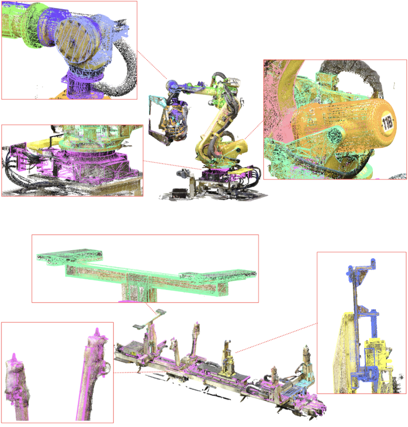
CAD models fitted to factory point clouds
1. Introduction
In automotive factories, moving equipment, such as articulated robots and conveyance systems, operate collaboratively to perform assembly tasks. These systems must operate without colliding with one another or surrounding structures. Traditionally, robot motion has been defined through manual “teaching,” in which an operator programs motion using a teach pendant or by physically guiding the robot. However, these procedures require stopping the production line, which makes downtime a critical concern. Moreover, the quality and efficiency of teaching depend heavily on operator skills, and continuous monitoring is required to avoid accidents.
To mitigate these issues, offline robot motion planning is essential prior to execution on actual machines. Constructing a high-fidelity virtual environment using point-cloud data is an effective solution for this problem. terrestrial laser scanners (TLSs) can capture accurate and dense 3D point clouds in factory environments, enabling robust collision detection. With these data, factory assets can be simulated within an as-is virtual environment that reflects a real workspace.
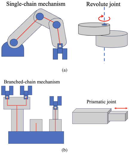
Fig. 1. Link mechanisms: (a) single-chain mechanisms, typical of articulated robots, are characterized by the sequential connection of links using revolute joints (rotational motion); and (b) branched-chain mechanisms, typical of conveyance systems, are characterized by multiple branching links incorporating prismatic joints (translational motion).
However, raw factory point clouds contain both stationary background structures and moving assets (robots, conveyors, and other equipment) that must be simulated. For effective motion planning, the static point clouds of these moving assets must be replaced with kinematic computer-aided design (CAD) models that support simulated motion. The link structure of the machine can be defined by a kinematic description format, such as the Unified Robot Description Format (URDF) 1, which accommodates both single-chain mechanisms with revolute joints (articulated robots) and branched-chain mechanisms with prismatic joints (conveyance systems), as shown in Fig. 1. Accurate registration between the CAD model and the point cloud is essential because pose estimation errors propagate directly into subsequent collision detection.
Many methods have been proposed for shape reconstruction from point clouds 2,3,4,5, and these techniques are effective for modeling static industrial parts. However, these methods assume a fixed underlying shape, and moving equipment such as articulated robots or conveyance systems are not satisfactory. The geometry of these machines changes with the joint configuration, making conventional reconstruction approaches unsuitable for recovering kinematically valid structures.
However, in industrial settings, manufacturers typically provide CAD models that explicitly represent the kinematic mechanisms of a machine. These models are constructed for motion definition and robot teaching and therefore consist of joint-separated components (links, sub-links, and actuated elements) organized so that each part can move independently in the simulation. Leveraging these structured CAD models provides a practical basis for single- and branched-chain mechanisms. By aligning each CAD component with the corresponding regions in the point cloud, the actual machine pose can be estimated while preserving its true kinematic structure.
However, several practical difficulties remain, even with these CAD models. Real TLS scans contain numerous nonmodeled components—wire harnesses, fasteners, hoses, and support brackets—that obscure the underlying machine geometry and degrade the registration accuracy. Moreover, articulated equipment often includes complex structures, such as multilink mechanisms, branched kinematic chains, and interchangeable end effectors. These factors make it challenging to obtain reliable alignment between CAD models and point-cloud observations in real factory environments.
To address these difficulties, this study proposes a robust and efficient fitting framework that integrates edge-weighted registration with fast edge detection tailored for organized TLS point clouds. By exploiting the scanning structure inherent in TLS measurements, this method accelerates edge extraction while effectively suppressing noise and outlier effects. The extracted edges are then incorporated into the registration process by assigning higher weights to the edge correspondences, thereby anchoring the alignment to geometrically reliable features that remain consistent between CAD models and real machines.
The remainder of this paper is organized as follows: Section 2 reviews related work. Section 3 describes the kinematic representation of articulated robots and conveyance systems using URDF. Section 4 presents a fast edge detection method tailored to organized TLS point clouds. Section 5 details the proposed edge-weighted registration for articulated robots. Section 6 extends this approach to conveyance systems with branched-chain mechanisms. Section 7 presents experimental results that verify the effectiveness of the proposed method, and Section 8 concludes the paper.
2. Related Work
2.1. CAD-Based Reconstruction and Fitting
Several CAD model–based fitting methods have been proposed for industrial robots.
Shah et al. 6 applied simulated annealing to fit multipart assembly models to point clouds and initialized the poses using oriented bounding boxes (OBB). However, real factory scans often contain nonmodeled elements, such as wire harnesses, bolts, and brackets, which distort the OBB and degrade the initialization accuracy. When the initial pose is inaccurate, the optimization may fail to converge to the global optimum.
Hu et al. 7 proposed a deep-learning-based framework using predefined CAD templates for object recognition and parameter estimation. Although effective under controlled conditions, articulated robots in automotive factories exhibit significant variations owing to their multiple links, subordinate components, closed-loop structures, and interchangeable end effectors. It is difficult to train a classifier that can accommodate all these variations.
Kawasaki et al. 8 introduced a fitting method for articulated robots; however, it required manual base-link initialization, increased the processing time, and increased the risk of human error. Their method also does not explicitly address nonmodeled components, resulting in unstable performance in real TLS scans. Furthermore, most existing fitting approaches implicitly assume single-chain link structures, limiting their applicability to the branched-chain mechanisms commonly found in conveyance systems.
2.2. ICP-Based Point-Cloud Fitting
The Iterative Closest Point (ICP) method 9 and its variants are among the most widely used methods for aligning two point clouds. Numerous extensions have been proposed; however, they share the common principle of iteratively estimating point correspondences and minimizing the geometric discrepancies between them. In its basic form, the ICP repeatedly assigns each point in the source cloud to the nearest point in the target cloud and computes the rigid transformation that best aligns the two sets.
Although effective for many rigid objects, the application of conventional ICP-based methods to articulated machines introduces several difficulties. First, ICP uniformly treats all points as equally informative, even though factory scans contain nonmodeled elements, such as wire harnesses, hoses, and fasteners, as well as occlusions and sensor noise. These factors generate geometric outliers that can significantly degrade the registration accuracy.
Second, ICP inherently assumes a single rigid body motion. By contrast, robots and conveyance systems consist of multiple links connected by joints, each of which requires its own motion. Independently estimating the pose of each link is challenging because naïvely applying ICP to individual parts can lead to inconsistencies between adjacent links. In articulated mechanisms, joint axes must remain coincident, and joint constraints must be satisfied; without incorporating such kinematic constraints, ICP solutions may violate the machine’s actual degrees of freedom or produce mechanically impossible configurations.
Finally, although many ICP variants attempt to mitigate noise and outliers, they still rely primarily on surface points that are heavily affected by nonmodeled attachments. In contrast, geometric edges, sharp intersections between links, or structural features, remain consistent between CAD models and real machines, making them more reliable cues for registration.
2.3. Edge Detection in Point Clouds
Point-cloud registration can be improved by exploiting geometric features rather than relying solely on the raw point positions. In this study, we focused on edge features that provide stable and distinctive geometric cues, even in cluttered factory environments. This section reviews existing methods for extracting edges from 3D point clouds and their applications to the registration process.
Extensive studies have been conducted on point-cloud edge detection. Hackel et al. 10 introduced a geometry-based contour detector to evaluate sharp changes in surface orientation; however, it relies on expensive 3D neighborhood searches and structured optimization. Pauly et al. 11 proposed a multiscale PCA-based technique for extracting line-type features from point-sampled surfaces. Although this method performs well for high-density and relatively clean data, its susceptibility to noise limits its effectiveness for real-world factory scans. More recently, Ben-Shabat and Gould 12 proposed DeepFit, which learns point-wise weights using a neural network, and applies weighted least squares for surface fitting. Although TLS is accurate and robust to density variations, the need to infer weights through a network introduces substantial computational costs, particularly for large-scale TLS point clouds.
In addition to feature extraction, several studies have leveraged linear features for point-cloud registration. Al-Durgham et al. 13 developed an automated random sample consensus (RANSAC)-based framework that exploits the invariant spatial separation and angular deviation between 3D line pairs to establish correspondences. Habib et al. 14 proposed a methodology that enforces the coincidence of conjugate linear features to integrate multisource data, including photogrammetric and LiDAR datasets, into a common reference frame. For large-scale urban environments, Stamos and Leordeanu 15 introduced a feature-based approach that organized segmented range data into a topological graph for scan placement. Furthermore, Date et al. 16 achieved efficient registration of bridge structures by employing a hash table-based RANSAC for an accelerated candidate search.
However, these existing approaches are primarily designed for static rigid objects and do not explicitly model the kinematic constraints of articulated or branched-chain industrial equipment. In contrast, our proposed method focuses on robust articulated model fitting by integrating explicit kinematic constraints with an edge-weighted registration framework, specifically addressing the challenge posed by nonmodeled components in real factory environments.
3. Kinematic Representation Using URDF
Several formats exist for representing link mechanisms in robotic systems, including graph-based models 17, multibody dynamics models 18, and the URDF. Graph-based methods capture the topological relationships between links and joints but often omit geometric details such as joint axes and precise poses, which are essential for tasks such as 3D model fitting. Multibody models support accurate dynamic simulations but tend to be complex and less intuitive for modular editing or visualization. Therefore, we adopted the URDF, which balances geometric expressiveness, structural simplicity, and wide compatibility. URDF is an XML-based format supported by ROS and is compatible with visualization and simulation tools (e.g., RViz 19 and Gazebo 20). A robot in URDF is represented as a tree of links and joints. Each joint specifies its type, axis, and relative pose, and the spatial relationship between the links is defined using XYZ translation and roll-pitch-yaw (RPY) rotation parameters. Fig. 2 illustrates a typical link-joint structure and its corresponding URDF.
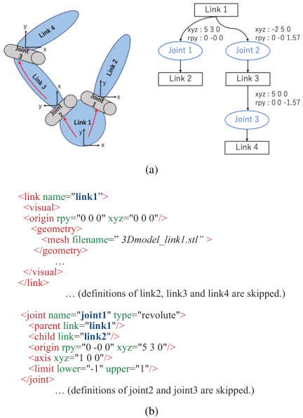
Fig. 2. Kinematic structure and URDF representation: (a) link-joint structure and (b) corresponding URDF.
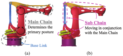
Fig. 3. URDF decomposition for closed-loop kinematics: (a) main chain (grey dashed outline) defining the primary posture and (b) sub-chain (pink dashed outline) moving in conjunction to satisfy the URDF tree structure requirement.
3.1. URDF of Articulated Robot
The URDF does not natively support closed-loop mechanisms. To represent articulated robots with such structures, we decompose the model into a main chain and one or more sub-chains, as shown in Fig. 3. This decomposition allows us to maintain a tree structure while modeling complex mechanisms.
We further modularized the model by separating the end effector (EEF) into its own URDF file. As EEFs vary in shape and function depending on the task, this separation allows for flexible reconfiguration. In factory environments, diverse robots can be constructed by combining a limited set of main-link structures with different EEFs. Reusing URDFs for the main chain, sub-chains, and EEFs simplifies the model construction, maintenance, and adaptation. Fig. 4(a) highlights this modular structure, in which the EEF is shown in red.
3.2. URDF of Conveyance System
These structured CAD models provide a practical basis for the development of branched-chain mechanisms with prismatic joints. The conveyance system has a simpler structure without closed loops. It consists solely of a main chain and can be represented using a single URDF. Fig. 4(b) shows the 3D assembly model of the conveyance system, demonstrating how the URDF encodes these branched-chain structures and their spatial relationships for 3D model fitting.
4. Fast Edge Detection from TLS Point Clouds
A major challenge in fitting is the presence of outliers. These include unmodeled artifacts, such as protective covers, wire harnesses, and other extraneous structures, which are absent from the CAD model and can severely degrade registration. Our approach is based on the observation that the edges of rigid structural components appear clearly and consistently in both the CAD model and TLS point clouds, whereas unmodeled objects such as covers or wire harnesses have irregular geometries and rarely form distinct edges. Accordingly, we extracted these stable structural edges and assigned them high weights during the registration. To achieve this, we introduce a fast edge-detection procedure that leverages the structured 2D grid representation of TLS data, which first computes high-quality normals, then identifies edge candidates based on normal consistency, and finally removes noise through region growth, as shown in the pipeline overview in Fig. 5.
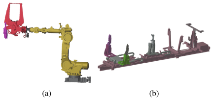
Fig. 4. Assembly models: (a) articulated robot and (b) conveyance system.
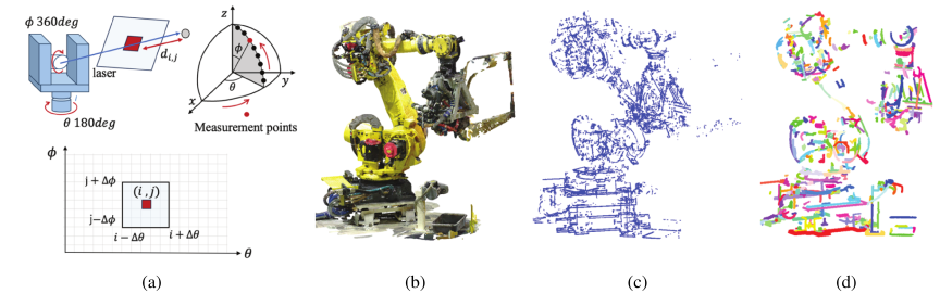
Fig. 5. Fast edge detection pipeline for TLS point clouds: (a) structured data acquisition by a TLS using polar coordinates \((\theta, \phi)\); (b) raw point cloud of an articulated robot; (c) extracted edge points; and (d) coherent structural edge segments after region growing.
4.1. Normal Estimation
The efficiency of the proposed method stems from leveraging the data structure inherent in TLS. A TLS captures points using a polar coordinate system based on azimuth (\(\theta\)) and elevation (\(\phi\)) angles, allowing the entire point cloud to be treated as a 2D array, \({P[i][j]}\) as shown in Fig. 5(a). This structure permits highly efficient neighborhood searches by accessing neighborhood pixels (\(P{[i\pm\Delta\theta]}{[j\pm\Delta\phi]}\)), which avoids computationally expensive 3D k-d tree searches. For each point \(\boldsymbol{p}_{i,j}\), we define an adaptive neighborhood on the 2D grid 21,22,23. The pixel radius (\(\Delta\theta\), \(\Delta\phi\)) scales inversely with the point’s distance \(d_{i,j}\) from the scanner. This ensures that the search window covers a consistent physical area and makes the estimation robust against density variations. Normal was computed in a two-stage process using weighted principal component analysis (WPCA) 24,25. First, the initial normal \(\boldsymbol{n}_{i,j}^{(0)}\) is computed. This WPCA assigns a greater influence to points \(\boldsymbol{p}_k\) closer to the center \(\boldsymbol{p}_{i,j}\), thereby enhancing robustness against noise. This is achieved using the following Gaussian weighting function, \(w_{\textrm{pca}}\), where \({h_{i,j}}^2\) is derived from the neighborhood’s spatial extent:
The parameter \(h_{i,j}\) is adaptively determined for each point as half the maximum Euclidean distance to its neighboring points within the local search window. To preserve sharp edges, only neighbors \(\boldsymbol{p}_k\) whose initial normals \(\boldsymbol{n}_k^{(0)}\) are sufficiently aligned with the central point’s initial normal \(\boldsymbol{n}_{i,j}^{(0)}\) are retained.
The alignment threshold \(\tau_{\textrm{align}}\) is determined empirically according to the expected noise level of the laser scanner to distinguish between noise and geometric discontinuities. A second WPCA is then performed on this filtered set to compute the final normal \(\boldsymbol{n}_{i,j}\), which preserves the sharp edges and prevents smoothing across discontinuities.
By leveraging the 2D grid, applying WPCA, and performing this two-step refinement, our method efficiently computed high-quality normals for both smooth surfaces and sharp edges, which are crucial for subsequent edge detection.
4.2. Edge Candidate Scoring
With accurate normals computed, the potential edge points are identified. Instead of comparing only immediately adjacent neighbors, we evaluated the normal consistency within an annular region around each point \(\boldsymbol{p}_i\). Neighborhood \(\mathcal{N}_i\) is defined as all points \(\boldsymbol{p}_k\) whose distance to \(\boldsymbol{p}_i\) satisfies
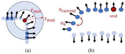
Fig. 6. Edge detection sub-steps: (a) annular neighborhood for edge candidate scoring and (b) normal consistency check for region-growing noise removal.
4.3. Region Growing for Noise Removal
Edge candidates can include noisy points. To extract coherent structural edges, all edge candidates from all scanner positions are aggregated into a kd-tree. The algorithm iterates through candidates sorted by edge score \(S_i\), selecting the first unassigned point \(p_{i}\) as the seed. Neighboring points within a radius are added to the current region only if their normals satisfy
Regions smaller than a minimum threshold \(\tau_{\textrm{min}}\) are discarded as noise. This process continues until all candidates are assigned to either a valid region or are removed.
Finally, edge weight \(w_{\textit{edge},i}\) is assigned to each point \(\boldsymbol{p}_i\). Points belonging to valid regions that remain after the noise removal process (exceeding \(\tau_{\min}\)) are assigned a high weight \(w_{\textit{high}}\), while all other points are assigned a base weight of 1:
The value of \(w_{\textit{high}}\) was determined through sensitivity analysis by varying the parameter from 2 to 100. The minimum pose error is obtained at \(w_{\textit{high}}=10\). Smaller values reduce the influence of the edge constraints, whereas excessively large values increase the sensitivity to noise at the detected edges. Therefore, \(w_{\textit{high}}=10\) was adopted as the default value in this study, although users can adjust this parameter when applying the method to different datasets.
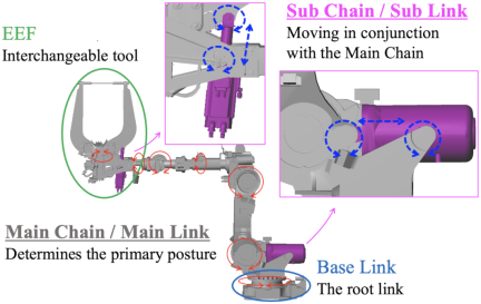
Fig. 7. Kinematic decomposition of an articulated robot. The articulated robot is decomposed into the base link, the main chain / main link, the sub chain / sub link, and the EEF.
5. Edge-Weighted Fitting of Articulated Robots
In this section, we describe a posture-estimation method for articulated robots composed of single-chain links with rotational joints, which are widely used in production lines. The overall structure of the articulated robot is illustrated in Fig. 7. The kinematic structure of each robot was defined using the URDF model, and the pose of each link was parameterized by its joint angle.
The proposed fitting pipeline consists of four stages: base-link fitting, main-link fitting, EEF fitting, and sub-link fitting. First, the base link was aligned with a point cloud. The remaining links were then fitted sequentially toward the EEF under the kinematic constraints specified in the URDF.
A key feature of this method is the use of edge weights computed in Eq. \(\eqref{eq:6}\) throughout all registration stages. These weights were incorporated into a weighted least-squares formulation for 6-DoF refinement and into a robust loss function for a 1-DoF joint angle search. This emphasizes stable geometric edges while suppressing flat regions and nonmodeled components, such as wire harnesses, enabling robust fitting under severe noise and occlusion.
Finally, the sub-links are estimated based on the propagated poses of the main links and the EEF.
5.1. Base Link Fitting
The base link defines the origin and coordinate systems of the entire robot. Accurate 6-DoF alignment (XYZ translation and RPY rotation) is essential because errors propagate to all subsequent links. The fitting process was divided into rough and precise registration phases.
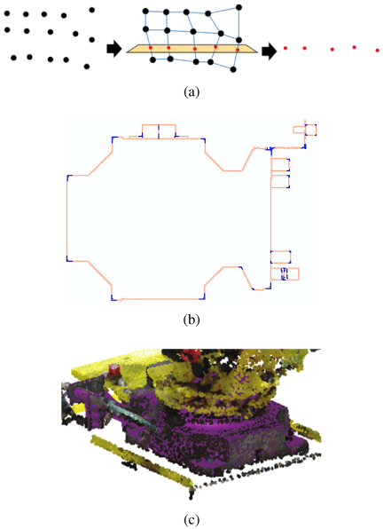
Fig. 8. Base link alignment steps: (a) the process of computing cross-sectional points by slicing the point cloud’s wireframe; (b) cross-sectional corners extracted from the Base link CAD model; and (c) fitting result of base link.
5.1.1. Rough Registration
The initial pose was estimated using a feature-based RANSAC 26 approach, assuming that the base link was installed horizontally. This method requires the extraction and matching of horizontal cross-sections from both the TLS point clouds and the CAD model.
We leverage the structured nature of the point cloud to generate a wireframe by connecting neighboring points and then compute the cross-sectional points by intersecting this wireframe with a horizontal plane, as shown in Fig. 8(a). Similarly, the cross section of the CAD model was obtained by slicing its polygonal edges.
High-curvature points (corners) were extracted from these cross sections. The local curvature at each point is approximated using the eigenvalues \(\lambda_0\) and \(\lambda_1\) (with \(\lambda_{0} > \lambda_{1}\)) of the PCA applied to its neighbors:
Points with curvatures significantly higher than the average are classified as corners, as shown in Fig. 8(b).
RANSAC was then applied to align the CAD model to the point cloud at the position where most of the corner points matched.
5.1.2. Precise Registration
A precise alignment was performed using weighted ICP, which assigns higher edge weights to structurally significant edge points to reduce the influence of outliers. In this case, the optimal rotation matrix \(\boldsymbol{R}\) and translation vector \(\boldsymbol{t}\) can be determined by solving the following optimization problem.
These weightings anchor the registration to structurally significant edges, ensuring that the final alignment is robust against outliers, as shown in Fig. 8(c).
5.2. Main Link Fitting
Once the base link (\(L_1\)) is fixed, the pose of each subsequent main link (\(L_k\), for \(k\ge 2\)) is determined sequentially. This process is not a 6-DoF registration but rather an estimation of the single 1-DoF joint angle (\(\theta_k\)) around the kinematically constrained axis defined in the URDF file. The sequential fitting process is shown in Fig. 9(a). This estimation was also performed at the rough and precise stages.
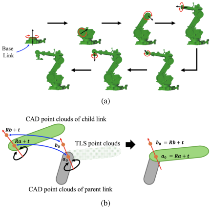
Fig. 9. Articulated robot fitting: (a) sequential fitting of single-chain links by estimating the revolute joint angle and (b) constraints on revolute joints.
5.2.1. Rough Registration (Rotational)
A robust search algorithm was employed to determine the approximate joint angle \(\theta_{k}\). The source CAD point clouds \(\mathcal{P}_k\) for link \(L_k\) were rotated around their joint axes at fixed angular intervals, stepping through the entire permissible range defined in the URDF. The total robustness loss was calculated at each step. The angle that yielded the minimum total loss was selected as the approximate estimate of \(\theta_k\).
This calculation requires finding the shortest distance from each transformed source point \(\boldsymbol{p}_i\in\mathcal{P}_k\) to the target cloud \(Q\). To perform this nearest-neighbor search efficiently, we leverage the 2D lattice of the TLS data (as described in Section 4.1) instead of a 3D search.
The loss function itself is designed to leverage the edge weights (\(w_{\textit{edge},i})\) while robustly handling the outliers. For each point pair with distance \(D\) and target edge weight \(w_{\textit{edge},i}\), the loss is defined based on an inlier threshold \(\tau_{\textrm{dist}}\):
For inliers, dividing by \(w_{\textit{edge},i}\) ensures that the stable edges guide the fitting. For outliers, the higher penalty \(\boldsymbol{D}\times w_{\textit{edge},i}\) effectively suppresses the influence of nonmodeled components (e.g., cables) by assigning them a high cost, ensuring that they do not lead to the optimization of incorrect poses.
The total loss for the angle, \(\textrm{Loss}(\theta_{k}) = \sum\textrm{Loss}_i\), is recorded. The angle \(\theta_k\) that minimizes this total loss is selected as the result of the rough search.
A known challenge arises with rotationally symmetric links, where this loss function \(\textrm{Loss}(\theta_{k})\) becomes ambiguous with respect to the joint angle. To resolve this, if link \(L_k\) is identified as symmetric, the loss function is modified to include the loss contribution from its child link \(L_{k+1}\). Since the child link \(L_{k+1}\) is typically asymmetric relative to the joint \(k\), its inclusion provides the necessary geometric constraint to find the unique, correct angle \(\theta_k\).
5.2.2. Precise Registration (Rotational)
The angle \(\theta_{k}\) obtained from the rough registration (Section 5.2.1) is used as the initial pose for the final refinement. We perform an axis-constrained Weighted ICP that optimizes the transformation (\(\boldsymbol{R}\), \(\boldsymbol{t}\)) by minimizing the following objective:
The first term is the edge-weighted point-to-point error, where \(w_{\textit{edge},i}\) is the edge weight derived from Eq. \(\eqref{eq:6}\). The second term enforces the kinematic constraint by penalizing the deviations between the transformed axis points of the child link \((\boldsymbol{a},\boldsymbol{b})\) and the corresponding axis points of the parent link \((\boldsymbol{a}_0,\boldsymbol{b}_0)\).
Following the optimization, the resulting rotation matrix \(\boldsymbol{R}\) must be converted back into the single scalar joint parameter \(\theta_{k}\). The final angle \(\theta_k\) is determined by projecting the optimized rotation \(\boldsymbol{R}\) onto the kinematically defined joint axis. This projection ensures that the final \(\theta_k\) strictly adheres to the 1-DoF rotational constraint, eliminating any residual numerical errors in pitch, yaw, or translation that may have persisted from the weighted least-squares solution.
The EEF also consisted of multiple links, as shown in Fig. 10. Because the EEF is connected to the end of the main link, its position and orientation are determined in the same manner based on the axial relationship with the previous link.
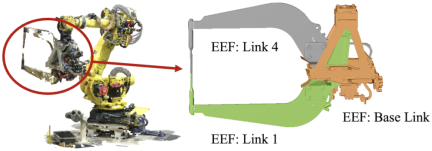
Fig. 10. EEF link structure.
5.3. Sub Link Fitting
The rotation angles of the sub-links can be uniquely determined from the rotation angles of the main links. The sub-link positions are computed as inverse kinematic solutions using the fixed main links.
6. Edge-Weighted Fitting of Conveyance System
This section describes the pose estimation method for conveyance systems, which, similar to articulated robots, are widely used in production lines and consist of branched-chain-connected links with prismatic joints. The proposed edge-weighted fitting method comprises two stages: base link and main link fitting.
6.1. Base Link Fitting
The conveyance system is equipped with multiple link mechanisms on top of the base link. To determine the position of the base link, feature points were extracted from both the TLS point clouds and the CAD model. Alignment was then performed by matching the corresponding feature points.
The conveyance system has upward-extending arms that hold the automobile parts in place. Therefore, the highest point of each arm is detected as a feature point.
To detect the feature points, a height map was generated by projecting the point cloud onto a horizontal grid, as shown in Fig. 11(a). Pixel value \(P_{(i,j)}\) represents the Z-coordinate (height) of the highest point in each grid cell. The feature points that were significantly higher than those of the surrounding pixels were selected.
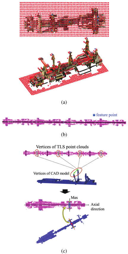
Fig. 11. Conveyance base link rough fitting: (a) height map generation from the point cloud; (b) feature point detection; and (c) center axis determination and feature matching for rough fitting.
Let the pixel value at \((i,j)\) be denoted as \(P_{(i,j)}\). The pixel values in the \(i\)-direction can be approximated by a second-order curve using the Taylor expansion, as shown in Eq. \(\eqref{eq:11}\).
Here, a larger value of \({\Delta^2 P}/{{\Delta i}^2}\) indicates a sharper convex shape, suggesting that the pixel corresponds to the vertex at the tip of the arm. The second-order difference between the pixels is computed as follows:
The same calculation was performed in the \(j\)-direction and along two diagonal directions. Using these results, the sharp convex vertices corresponding to the arm tip are detected as pixels that satisfy the following condition, where \(T\) is the negative threshold for convex detection:
The detected feature points are indicated in blue in Fig. 11(b). Next, the center axis of the conveyance system was determined based on these feature points. The central axis is computed to maximize the symmetry of the feature points. When a pair of symmetrical feature points was selected, the axis was set perpendicular to the line connecting them. To estimate the symmetry axis, the RANSAC method was used to determine the axis that maximized the number of symmetrical feature points. The detected center axis is shown in Fig. 11(b). Feature points that did not exhibit symmetry with respect to the central axis were excluded.
Feature points were extracted from the CAD model as vertices with large Z-coordinates. In the rough fitting process, the distances between pairs of symmetrical feature points were calculated, and the corresponding pairs were identified between the CAD model and point cloud. Once the corresponding pairs were determined, a rough fitting was performed by aligning them, as shown in Fig. 11(c).
Through rough fitting of the CAD model, the points around the base link can be extracted from the point cloud. Subsequently, an accurate fitting was achieved by applying a weighted ICP (Section 5.1.2) to align the CAD point clouds with the TLS point clouds. Here, the edge weight \(w_{\textit{edge},i}\) is the weight derived from the edge detection results in Eq. \(\eqref{eq:6}\).
6.2. Main Link Fitting
Once the base link was fixed, the pose of each subsequent main link was determined. The sequential fitting process and geometric constraints for the branched-chain mechanism are shown in Fig. 12. In conveyance systems, these links typically move along a 1-DoF prismatic (translational) axis, as defined in the URDF. As in the case of the articulated robot, the fitting process was performed at the rough and precise stages.
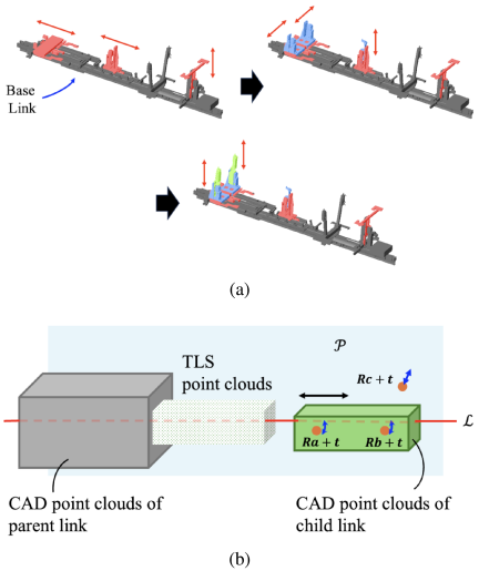
Fig. 12. Conveyance system fitting: (a) sequential fitting of branched-chain mechanisms by estimating the prismatic joint translation and (b) constraints on prismatic joints.
6.2.1. Rough Registration (Prismatic)
First, the approximate translational position \(d_k\) was determined. The fitting process is iterated through the permissible translational range of the joint at fixed intervals.
At each discrete step \(d_k\) along the joint axis, the total Robust Loss is calculated using an identical edge-weighted loss function (Eq. \(\eqref{eq:9}\)), as described in Section 5.2.1. The translational position \(d_{k}\) that yields the minimum total loss is selected as the initial pose for the next step.
To handle branched kinematic chains, the pose of each link is recursively calculated by tracing its parents back to the fixed base link before the loss is computed. For computational efficiency, the nearest-neighbor search required for this loss calculation also leveraged the 2D lattice of the TLS data (Section 4.1).
6.2.2. Precise Registration (Prismatic)
The translational parameter \(d_{\textrm{rough}}\) from the rough registration (Section 6.2.1) was used as the initial pose for the final refinement.
Unlike a revolute joint, where the link position is fixed at a point, a prismatic joint permits translation along the joint axis while maintaining the link collinear with that axis. Therefore, we constrained certain link points to geometric primitives (point-to-line and point-to-plane) instead of fixing them to the target coordinates.
We perform a constrained weighted ICP that optimizes the transformation \((\boldsymbol{R},\boldsymbol{t})\) by minimizing
To ensure that the result strictly adheres to the axis, the scalar joint parameter update \(d_k\) was determined by projecting the optimized translation vector \(\boldsymbol{t}\) onto the normalized joint axis unit vector.
7. Evaluation Results
This section presents qualitative and quantitative evaluations of the proposed edge-weighted registration method. As the true pose of the robot is unknown in real factory point clouds, a quantitative assessment was performed using virtual point clouds generated from CAD models via a simulated laser scanner.
The following parameters for edge detection and registration were consistently applied across all experiments: the alignment threshold \(\tau_{\textrm{align}}=0.866\) (corresponding to \(\cos 30°\)) (Eq. \(\eqref{eq:2}\)), scoring neighborhood \(r_{\min}=5.0\) mm and \(r_{\max}=10.0\) mm (Eq. \(\eqref{eq:3}\)), the region-growing threshold \(\tau_{\textrm{region}}=0.95\) (Eq. \(\eqref{eq:5}\)), and the minimum region size \(\tau_{\min}=300\) points (Section 4.3). The high weight \(w_{\textit{high}}\) for identified edge points was set to 10 (Eq. \(\eqref{eq:6}\)).
7.1. Qualitative Evaluation on Real Factory Point Clouds
The proposed method was applied to point clouds captured at an automotive factory. The input point clouds for the articulated robot and conveyance system contained approximately 5.5 million and 5.0 million points, respectively. The average point spacing (grid resolution), calculated as the mean distance to the nearest neighbor across all valid points, was approximately 1.66 mm for the articulated robot and 1.60 mm for the conveyance system. The OBB size was approximately \(\mbox{2.5~m} \times \mbox{2.0~m} \times \mbox{2.5~m}\) for the articulated robot, and \(\mbox{1.6~m} \times \mbox{1.7~m} \times \mbox{5.5~m}\) for the conveyance system. These datasets contain significant sensor noise, occlusions, and numerous nonmodeled accessories such as wire harnesses and covers, which act as geometric outliers. Despite these challenges, the method successfully aligned the CAD models of both articulated robots and conveyance systems, as shown in Fig. 13. By assigning high weights to stable geometric edges, the influence of nonmodeled components was effectively suppressed, allowing for accurate reconstruction of kinematically valid 3D assembly models.
To evaluate the effect of the edge-weighting strategy, we compared our approach with a conventional unweighted registration method using point clouds acquired from real robots (Fig. 14). In the unweighted case, small fitting errors in individual links accumulate along the kinematic chain, leading to a significant misalignment of the robot’s EEF. By contrast, the edge-weighted method anchors each registration step to reliable geometric features, effectively minimizing the cumulative error and ensuring precise alignment, even at the extremities of the machine.
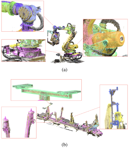
Fig. 13. Fitting results on factory point clouds: (a) articulated robot with fitted CAD model and (b) conveyance system with fitted CAD model.
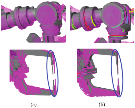
Fig. 14. Registration on real point clouds: (a) unweighted (cumulative error at robot tip) and (b) edge-weighted (reduced cumulative error).
7.2. Computational Efficiency
The efficiency of the proposed method was evaluated using a desktop PC equipped with an Intel Core i9-10900K CPU @ 3.70 GHz and 62.7 GiB RAM. The processing times for both target systems are summarized as follows:
-
Articulated robot: Edge detection took 9.9 s, base-link registration required 296.7 s, and sequential fitting (main/sub-chains and EEF) was completed in 12.6 s.
-
Conveyance system: Edge detection took 10.0 s, base-link registration required 143.0 s, and sequential fitting was finished in 37.3 s.
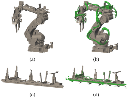
Fig. 15. Virtual CAD models: (a) articulated robot without accessories (UW condition); (b) articulated robot with accessories (EW condition); (c) conveyance system without accessories (UW condition); and (d) conveyance system with accessories (EW condition).
Base-link registration is the most time-consuming stage because it involves a RANSAC-based global search and feature matching to establish an initial coordinate system. However, the subsequent link-by-link pose estimation is significantly accelerated by leveraging the structured 2D grid of the TLS data for efficient neighbor searching.
These results demonstrated that the proposed method is computationally practical for processing large-scale point clouds in factory environments.
7.3. Quantitative Evaluation Setup
We assessed the robustness of the method using virtual point clouds generated from CAD models. The virtual datasets for the articulated robot and conveyance system consisted of approximately 4.7 million and 7.3 million points, respectively. The average point spacing was approximately 1.7 mm for the articulated robot and 2.36 mm for the conveyance system, respectively. This evaluation used three unique postures for both the articulated robot and the conveyance system. For each instance, we generated two datasets: one without and one with nonmodeled accessories (e.g., wire harnesses and covers). Fig. 15 shows the virtual CAD models. To simulate real acquisition artifacts, we nonuniformly placed virtual laser scanners to induce occlusions and applied Gaussian noise (\(\sigma=1\) mm) along the laser irradiation direction to the resulting point clouds. Fig. 16 illustrates the virtual data acquisition setup and the resulting noisy point cloud details.
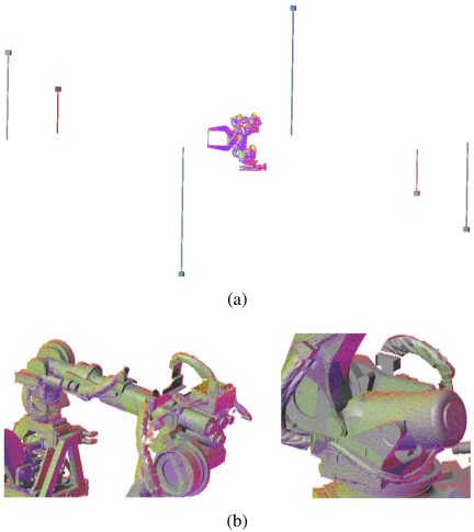
Fig. 16. Virtual data acquisition: (a) virtual laser scanner and (b) virtual point clouds.
7.4. Quantitative Results and Discussion
The errors in the rotational angles of the articulated robot and translational distances of the conveyance system are summarized in Tables 1 and 2, respectively. Under the “With Accessories” condition, the proposed edge-weighted precise fitting consistently achieved the lowest average error compared with the unweighted approach. These results demonstrate that assigning high weights to structural edges effectively suppresses interference from nonmodeled components, thereby significantly improving the robustness of posture estimation for both single-chain and branched-chain link mechanisms.
Although the observed accuracy improvements might appear marginal, they are critical for large-scale industrial systems where minor pose errors are amplified along extended kinematic chains. For the articulated robot in this study (overall height \(\approx 2.5\) m), the EEF extends approximately 1.0 m from the final joint to the welding tip. An angular error of merely 0.1° at the joint level thus results in a positional deviation of \(L\times \theta\approx 1.75\) mm at the tooltip. Such joint-level inaccuracies accumulate millimeter-scale endpoint errors, which are significant in precision-critical manufacturing. Similarly, in the 5.5 m long conveyance system, minor axis misalignments led to amplified deviations at the tips of the arm segments. Consequently, submillimeter pose accuracy is indispensable for high-fidelity virtual environments to ensure reliable collision detection and safe motion planning.
Table 1. Rotational angle error (in degrees) for articulated robot joints.

Table 2. Translational distance error (in millimeters) for conveyance system joints.

8. Conclusion
This study proposes a robust edge-weighted registration methodology for accurately aligning the CAD models of articulated robots and conveyance systems with noisy TLS point clouds. It incorporates a fast edge-detection algorithm that exploits the structured nature of TLS data to identify stable geometric edges. By assigning higher weights to these edges during registration, the method effectively suppressed the influence of irregular nonmodeled components (outliers) and achieved a robust alignment. This approach uniformly accommodates both single-chain link mechanisms and branched-chain mechanisms using URDF. A quantitative evaluation using simulated data demonstrated that edge-weighted registration significantly improved the robustness and accuracy of pose estimation, particularly when nonmodeled components were present.
- [1] D. Tola and P. Corke, “Understanding URDF: A survey based on user experience,” 2023 IEEE 19th Int. Conf. Autom. Sci. Eng. (CASE), 2023. https://doi.org/10.1109/CASE56687.2023.10260660
- [2] M. Berger et al., “A survey of surface reconstruction from point clouds,” Comput. Graph. Forum, Vol.36, No.1, pp. 301-329, 2017. https://doi.org/10.1111/cgf.12802
- [3] M. Kazhdan, M. Bolitho, and H. Hoppe, “Poisson surface reconstruction,” Eurogr. Symp. Geom. Process., pp. 61-70, 2006. https://doi.org/10.2312/SGP/SGP06/061-070
- [4] Y. Li et al., “GlobFit: Consistently fitting primitives by discovering global relations,” ACM Trans. Graph., Vol.30, No.4, Article No.52, 2011. https://doi.org/10.1145/2010324.1964947
- [5] R. Schnabel, R. Wahl, and R. Klein, “Efficient RANSAC for point-cloud shape detection,” Comput. Graph. Forum, Vol.26, No.2, pp. 214-226, 2007. https://doi.org/10.1111/j.1467-8659.2007.01016.x
- [6] G. A. Shah, A. Polette, J.-P. Pernot, F. Giannini, and M. Monti, “Simulated annealing-based fitting of CAD models to point clouds of mechanical parts’ assemblies,” Eng. Comput., Vol.37, No.4, pp. 2891-2909, 2021. https://doi.org/10.1007/s00366-020-00970-8
- [7] S. Hu, A. Polette, and J.-P. Pernot, “SMA-Net: Deep learning-based identification and fitting of CAD models from point clouds,” Eng. Comput., Vol.38, No.6, pp. 5467-5488, 2022. https://doi.org/10.1007/s00366-022-01648-z
- [8] K. Kawasaki, K. Takeda, and H. Masuda, “Extraction and reconstruction of articulated robots from point clouds of manufacturing plants,” Comput.-Aided Des. Appl., Vol.22, No.4, pp. 616-628, 2025. https://doi.org/10.14733/cadaps.2025.616-628
- [9] K. S. Arun, T. S. Huang, and S. D. Blostein, “Least-squares fitting of two 3-D point sets,” IEEE Trans. Pattern Anal. Mach. Intell., Vol.PAMI-9, No.5, pp. 698-700, 1987. https://doi.org/10.1109/TPAMI.1987.4767965
- [10] T. Hackel, J. D. Wegner, and K. Schindler, “Contour detection in unstructured 3D point clouds,” 2016 IEEE Conf. Comput. Vis. Pattern Recognit., pp. 1610-1618, 2016. https://doi.org/10.1109/CVPR.2016.178
- [11] M. Pauly, R. Keiser, and M. Gross, “Multi-scale feature extraction on point-sampled surfaces,” Comput. Graph. Forum, Vol.22, No.3, pp. 281-289, 2003. https://doi.org/10.1111/1467-8659.00675
- [12] Y. Ben-Shabat and S. Gould, “DeepFit: 3D surface fitting via neural network weighted least squares,” arXiv:2003.10826, 2020. https://doi.org/10.48550/arXiv.2003.10826
- [13] K. Al-Durgham, A. Habib, and E. Kwak, “RANSAC approach for automated registration of terrestrial laser scans using linear features,” ISPRS Ann. Photogramm. Remote Sens. Spat. Inf. Sci., Vol.II-5/W2, pp. 13-18, 2013. https://doi.org/10.5194/isprsannals-II-5-W2-13-2013
- [14] A. Habib, M. Ghanma, M. Morgan, and R. Al-Ruzouq, “Photogrammetric and lidar data registration using linear features,” Photogramm. Eng. Remote Sens., Vol.71, No.6, pp. 699-707, 2005. https://doi.org/10.14358/PERS.71.6.699
- [15] I. Stamos and M. Leordeanu, “Automated feature-based range registration of urban scenes of large scale,” 2003 IEEE Comput. Soc. Conf. Comput. Vis. Pattern Recognit., Vol.2, pp. II-555-II-561, 2003. https://doi.org/10.1109/CVPR.2003.1211516
- [16] H. Date et al., “Efficient registration of laser-scanned point clouds of bridges using linear features,” Int. J. Automation Technol., Vol.12, No.3, pp. 328-338, 2018. https://doi.org/10.20965/ijat.2018.p0328
- [17] F. Lu and E. Milios, “Globally consistent range scan alignment for environment mapping,” Auton. Robots, Vol.4, No.4, pp. 333-349, 1997. https://doi.org/10.1023/A:1008854305733
- [18] P. E. Nikravesh and H. A. Affifi, “Construction of the equations of motion for multibody dynamics using point and joint coordinates,” M. F. O. Seabra Pereira and J. A. C. Ambrósio (Eds.), “Computer-Aided Analysis of Rigid and Flexible Mechanical Systems,” pp. 31-60, Springer, 1994. https://doi.org/10.1007/978-94-011-1166-9_2
- [19] H. R. Kam, S.-H. Lee, T. Park, and C.-H. Kim, “RViz: A toolkit for real domain data visualization,” Telecommun. Syst., Vol.60, No.2, pp. 337-345, 2015. https://doi.org/10.1007/s11235-015-0034-5
- [20] N. Koenig and A. Howard, “Design and use paradigms for Gazebo, an open-source multi-robot simulator,” 2004 IEEE/RSJ Int. Conf. Intell. Robots Syst., Vol.3, pp. 2149-2154, 2004. https://doi.org/10.1109/IROS.2004.1389727
- [21] H. Masuda and I. Tanaka, “Extraction of surface primitives from noisy large-scale point-clouds,” Comput.-Aided Des. Appl., Vol.6, No.3, pp. 387-398, 2009. https://doi.org/10.3722/cadaps.2009.387-398
- [22] H. Masuda, T. Niwa, I. Tanaka, and R. Matsuoka, “Reconstruction of polygonal faces from large-scale point-clouds of engineering plants,” Comput.-Aided Des. Appl., Vol.12, No.5, pp. 555-563, 2015. https://doi.org/10.1080/16864360.2015.1014733
- [23] A. Chida and H. Masuda, “Reconstruction of polygonal prisms from point-clouds of engineering facilities,” J. Comput. Des. Eng., Vol.3, No.4, pp. 322-329, 2016. https://doi.org/10.1016/j.jcde.2016.05.003
- [24] H. Hoppe, T. DeRose, T. Duchamp, J. McDonald, and W. Stuetzle, “Surface reconstruction from unorganized points,” Proc. 19th Annu. Conf. Comput. Graph. Interact. Tech., Comput.-Aided Des. Appl. (SIGGRAPH), pp. 71-78, 1992. https://doi.org/10.1145/133994.134011
- [25] D. Levin, “Mesh-independent surface interpolation,” G. Brunnett, B. Hamann, H. Müller, and L. Linsen (Eds.), “Geometric Modeling for Scientific Visualization,” pp. 37-49, Springer, 2004. https://doi.org/10.1007/978-3-662-07443-5_3
- [26] M. A. Fischler and R. C. Bolles, “Random sample consensus: A paradigm for model fitting with applications to image analysis and automated cartography,” Commun. ACM, Vol.24, No.6, pp. 381-395, 1981. https://doi.org/10.1145/358669.358692
This article is published under a Creative Commons Attribution-NoDerivatives 4.0 Internationa License.