Technical Paper:
Development of a Computer-Aided Testing System for 3D Coordinate Measuring Machine
Naoki Asakawa*,†
 , Daiju Hoya*, Keigo Takasugi*, and Borja de la Maza**
*Kanazawa University
Kakuma-machi, Kanazawa, Ishikawa 920-1192, Japan
†Corresponding author
**Trimek S.A.
Altube-Zuia, Spain

Three-dimensional (3D) measurement systems are widely used in the machinery industry, and the measuring range has expanded with the popularization of optical probes. As measurement results are highly dependent on the scanning path, a computer-aided testing (CAT) system is developed to automatically generate a scanning path from the computer-aided design (CAD) data of the target. However, in the case of line laser probes, which are commonly used as optical probes, it is necessary to generate scanning paths considering the shape variations along the scanning lines based on the scanning posture. Furthermore, using probes with a wide measurement area, such as a line laser probe, causes overlaps, i.e., the duplication of the measurement areas. Reducing overlaps is required because they cause deterioration of the quality of point-cloud data and increase the amount of data. Focusing on a 3D measurement system using a line laser probe, this study developed a path generation system to automatically create scanning paths from the CAD data of a target and a measurement simulator to detect overlaps. This study presents the measurement results obtained using the scanning paths generated by the proposed CAT system and compares the results of simulations with those of actual measurements.
1. Introduction
Recently, product shapes have become complicated because of the development of new technologies, such as metal additive manufacturing and multitasking machines 1,2. Furthermore, machining accuracy has improved with the development of machining technologies 3. Consequently, not only design and manufacturing processes but also inspection processes are becoming increasingly important, and measurement technology is advancing 4,5. These manufacturing processes are primarily managed using digital data. First, after designing using computer-aided design (CAD) and computer-aided engineering, the design data are used in computer-aided manufacturing. Next, the products are inspected and evaluated by computer-aided testing (CAT) using a coordinate measuring machine (CMM). Finally, the shape information is digitized and fed back into design and manufacturing processes. By building such a cycle, it is possible to compare the CAD data with the manufactured shape data, thereby reducing production time and improving quality 6,7. In this cycle, a three-dimensional (3D) measurement system is used and includes sensor probes that obtain measurement points by approaching the object surface and positioning mechanisms that control the position and posture of the probe.
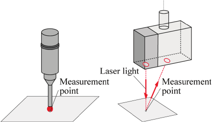 (a) Contact type(b) Non-contact type
Fig. 1. Sensor probe.
The positions of the target objects are obtained using a sensor probe. Sensor probes are classified into contact (Fig. 1(a)) and non-contact types (Fig. 1(b)). The contact type obtains positions by contacting the object with a sphere attached to the tip of the mechanical stylus. This type has the advantage of high-accuracy measurements and the disadvantage of extremely low measurement efficiency. The non-contact method obtains coordinates using the reflection of light or ultrasonic waves. Accordingly, optical 3D measurements have attracted significant attention because they enable wide-area, high-speed optical probes 8.
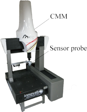
Fig. 2. 3D measurement system.
In optical 3D measurements, the surface shapes are obtained as point clouds consisting of a set of 3D positions. The line laser probe, which constitutes much of the noncontact type, can obtain positions immediately from the reflection of laser light. This type has the advantage of obtaining a large amount of point data in a short time and the disadvantage of low accuracy compared to the contact type 9. This study used a non-contact optical probe to achieve wide-area and high-speed measurements. The optical probes were classified according to the measurable areas in a single scan. They can be classified into three types based on the size of the measurement area: point type, line type, and area types. The point-type and line-type require continuous positioning, whereas the area-type does not. Therefore, as the measurement area increases, the measurement efficiency increases. However, the line and area types require hundreds to thousands of measurement points for each measurement. Therefore, they have the disadvantages of producing unnecessary measurement data and difficulty adapting to variations in shape. Accordingly, line-type optical probes tend to be used in 3D measurements to increase measurement efficiency and adapt to target shapes.
The position and posture of the probe are controlled using a positioning mechanism, as shown in Fig. 2. In the case of highly accurate measurements, the CMM can measure more accurately than articulated robots. Therefore, CMMs are commonly used in inspection processes. However, the quality of the scanning path depends on the operator.
Therefore, this study constructed a 3D measurement system with a line laser probe as the sensor and a CMM as the positioning mechanism.
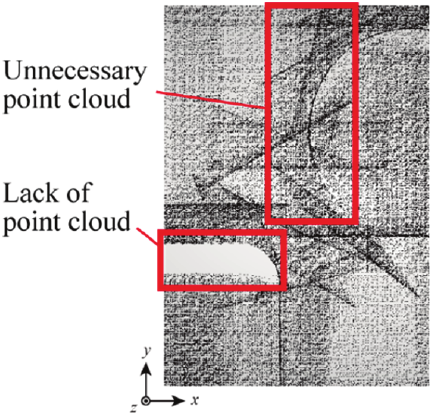
Fig. 3. Low-quality point cloud data.
In this 3D measurement system, it is impossible to obtain the shape information of the entire target with a single positioning operation. Therefore, to measure target areas, it is necessary to repeatedly conduct measurements while adjusting the position and posture of the probe to match the target shape for each measurement. However, manual generation of scanning paths by operators using line-type probes is extremely difficult. In addition, measuring with inappropriate scanning paths causes unnecessary or insufficient point cloud acquisition, as shown in Fig. 3. Therefore, the quality of point-cloud data decreases. Accordingly, because the obtained point cloud data depend on the posture and path at the time of measurement, automating scanning-path generation is desired. Thus, various approaches have been proposed, including the CAT system, which automatically generates measurement programs based on measurement items, and the method of planning paths based on CAD models 10,11.
Phan et al. focused on the increase in measuring time and decrease in measurement accuracy due to the overlap caused by measurements using a line laser probe. They developed a path generation system with six-axis robot-installed overlap control 12. The overlap is caused by the duplication of the measurement areas of neighboring scanning paths, leading to variations in the measurement point cloud density. Consequently, this results in an increase in unnecessary data capacity and errors in the geometric shape extraction 13. Because these overlaps negatively influence inspection after measurement and reverse engineering, minimizing the overlap is desirable. However, in a five-axis CMM, owing to the constraints described in Section 3.3, it is necessary to consider that the scanning posture cannot be changed until the measurement along a single linear scanning path is completed.
Accordingly, this study developed a 3D measurement system using a line laser probe. The CAT system comprised the following two components. The first component was a path-generation system that generated a scanning path and posture from the CAD data of the target. The second component was a measurement simulator that detected the overlapping parts caused by the generated scanning paths. Thus, this paper reports a measurement evaluation using scanning paths generated by the proposed CAT system and a comparison evaluation between the overlap results detected by the simulator and actual measurement results.
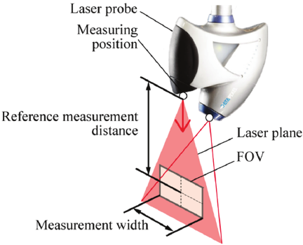
Fig. 4. Line laser probe.
2. CAT System
2.1. Overview of CAT System
This study used a bridge-type CMM (Innovalia Metrology, Spark gage 06.05.05) as the positioning mechanism and a line laser probe (Datapixel, Optiscan 1040-L) as the optical probe. The CAT system comprised a path generation system and measurement simulator for shape measurements. Kodatuno, a geometric calculation library for path generation systems 14, and a PC configured with an Intel Core i7-8700 CPU, Nvidia GeForce RTX 2060 GPU, and 16 GB of memory were used for simulations.
2.2. Bridge-Type CMM
The CMM has five axes: three orthogonal axes and two rotational axes. The operating range of the three orthogonal axes is 600 \(\times\) 500 \(\times\) 500 mm. In addition, the CMM has an inclined axis and a rotational axis for posture control. The operating range of the inclined axis is \(-180°\) to 180° and that of the rotational axis is 0° to 105°. The inclination and rotational angles were set at intervals of 7.5°. In addition, the measurement accuracy was independent of the temperature changes.
2.3. Line Laser Probe
The line laser probe shown in Fig. 4 uses a diffuse-reflection-based detection method and a triangulation-based measurement principle. The characteristics of the used probe are a maximum measurement width of 40 mm and a measurement distance of \(93\pm 20\) mm from the laser emission unit. The measurable area (field of view) was defined as the rectangular area obtained based on the measurement width and distance. In addition, the measurement accuracy is \(\pm 10\) μm.
2.3.1. Diffuse Reflection Type
The laser light emitted from the probe is reflected onto the surface of the object. Specular reflection is the primary component of mirror surfaces. However, diffuse reflection is the primary component of a general surface 15,16. As most mechanical parts are general surfaces, we used a diffuse reflection type.
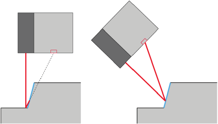
 (a) Incident light(b) Reflected light
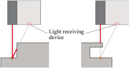
Fig. 5. Occurrence of occlusion.
2.3.2. Triangulation
The laser light emitted from the emitting section is shaped into a line through an emitter lens and projected onto the object. Subsequently, the diffusely reflected laser light is imaged onto a light-receiving device through a receiver lens. Triangulation was used to calculate the amount of change in the imaging position and measurement distance. Using this method, we can obtain the relative coordinates of the measured point and probe 17.
3. Constraints of Path Generation
3.1. Overview of Constraints
In a path generation system, the scanning paths are regarded as repetitions of the relative positioning of the probe against the target surface. This positioning is determined by the relative distance and angle and is closely related to the quality of measured data. In general, the reference measurement distance is ideal for the relative distance, and the posture perpendicular to the measured surface is ideal for the relative angle 18. Furthermore, constraints were imposed on the path-generation system by the equipment.
3.2. Constraints by Probe
Constraints (1)–(3) must be considered based on the measurement principles of the probe. In this context, the triangle connected to the scanning line and the position of laser incidence is defined as the laser plane, as shown in Fig. 4.
-
(1)
Probe positioning such that the measured surface falls within the field of view (FOV).
-
(2)
Probe positioning that prevents occlusion.
-
(3)
Scanning direction set along the normal vector to the laser plane.
In (1), the range can be detected when the laser light is limited by the probe specifications. Therefore, the probe must be positioned such that the measured surface falls within the defined FOV. In (2), the reflected laser light must be detected by light-receiving devices, as shown in Fig. 5. Therefore, occlusion must not occur in either the incident or reflected direction. In addition, it is desirable to consider the scanning direction, as described in (3).
3.3. Constraints by Position Mechanism
During the measurement, the positioning mechanism controls the position and posture of the probe. Therefore, it is necessary to consider constraints (4) and (5).
-
(4)
The posture of the probe cannot be changed during the measurement.
-
(5)
The probe posture cannot be controlled around the posture vector D\(_{\textrm{k}}\), which represents the direction of the laser emission.
Regarding (4), a change in posture should be avoided to prevent deterioration of the measurement accuracy of the CMM. Regarding (5), perfect control of the posture of the line laser probe requires three degrees of freedom; however, the system controls probe posture using only two rotational axes of the CMM in this study.
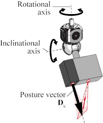
Fig. 6. Posture vector.
4. System
4.1. Overview of Path Generation
This system automatically generates a scanning path by loading the shape data of the measurement target and selecting the surface for measurement. This information included occlusion occurrence, and measurement accuracy was evaluated for each surface. Subsequently, a measurement position was generated for each surface based on this information. Additionally, a measurement position was generated for each posture. This method can be applied to free-form surfaces that fit within an FOV. Even if the surface is not fit within the FOV, the method can be applied by changing the scanning posture and dividing into multiple scanning paths.
4.2. Determination of Measurement Posture
As shown in Fig. 6, the measurement posture can be expressed by the posture vector D\(_{\textrm{k}}\) based on the rotation and inclination angles. Because each angle can be set at intervals of 7.5°, D\(_{\textrm{k}}\) was determined from 49 rotation-angle candidates \(\times\) 15 inclination candidates. In this system, areas that cannot be measured based on the occurrence of occlusions were defined on the target surface. An appropriate posture was selected for each measurable surface. First, judgment points were generated on the target surface, as shown in Fig. 7. The judgment vectors N\(_{\textrm{k}}\) were generated in the direction normal to the target surface from the judgment point. The distance between the judgment points was determined to be smaller than the point distance per irradiation, which was determined based on the measurement period and scanning speed. Then, one judgment point was selected, and intersections with the straight line in the N\(_{\textrm{k}}\) direction and each surface were checked.
When an intersection is detected, interference between the surface and the rest of the straight line in the D\(_{\textrm{k}}\) direction was carried out.
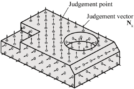
Fig. 7. Judgment points and vector.
If interference is detected in all straight lines in the D\(_{\textrm{k}}\) direction, this judgment point is regarded as a point that cannot be measured due to occlusion occurrence and is deleted.
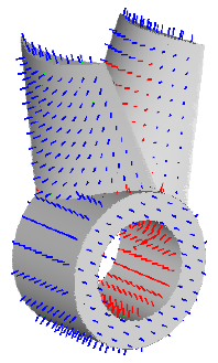
Fig. 8. Occlusion occurrence.
The target shape when the occlusion occurs is shown in Fig. 8. The measurable vectors are shown in blue, and the unmeasurable vectors are shown in red. The angles between N\(_{\textrm{k}}\) and D\(_{\textrm{k}}\) are then calculated at the remaining judgment points. If the calculated angle is less than or equal to 45°, the judgment point is regarded as a measurable point at this D\(_{k}\). This process was applied to all D\(_{\textrm{k}}\), and the D\(_{\textrm{k}}\) with the most measurable points was selected as the measurement posture at the surface. In the case where multiple measurement postures have the same number of measurable points, the one with the smaller angle between D\(_{\textrm{k}}\) and the average of N\(_{\textrm{k}}\) was selected as the measurement posture. This process was repeated for all the judgment points on the target surfaces. Even when occlusion occurs in a certain posture, the target can be measured by changing the posture. An example of this is shown in Fig. 9.
 (a) Unmeasurable(b) Measurable
Fig. 9. Scanning posture.
Fig. 10. Division of measurement.
4.3. Division of Measurement Surface
The target surfaces were divided for each selected posture in the measurement domain as shown in Fig. 10. An offset point was generated. The distance between this point and the measurable judgment point was equal to the reference measurement distance in the direction of the posture vector. A plane was generated with its normal vector aligned with D\(_{\textrm{k}}\) of the measurement posture. The distance between the generated plane and other measurable points was then calculated. If this distance was less than the reference measurement distance of the probe, then the other measurable point belonged to the same measurement domain as the other measurable point. Otherwise, a new plane was generated for the measurable point belonging to the new measurement domain.
4.4. Generation of Scanning Path
Scanning paths were generated to comprehensively cover the measurable points in each generated measurement domain. In this context, considering constraint (3), the scanning paths were set as straight lines. Furthermore, when multiple target surfaces or multiple measurement domains exist, the intermediate path along the \(Z\)-axis and the connection path connecting to the nearest measurement scanning path were used to construct a single-path stroke. When using the shape shown in Fig. 7, a scanning path can be generated within 3 min.
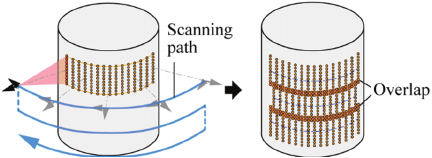
Fig. 11. Overlap.
5. Overlap
5.1. Overview of Overlap
When using a 3D measurement system, duplication of the measurement area occurs because of various factors. Examples include the wide measurement area of the probe and division of the scanning path into several paths. In the study, duplication of the measurement area, defined as “overlap,” is shown in Fig. 11. The overlap helps avoid areas lacking point clouds. However, various problems are caused by this overlap, as mentioned below. Accordingly, it is desirable to reduce the overlapping parts and limit the point-cloud density to satisfy the requirements.
5.2. Problems
Problems caused by the occurrence of overlap are variations in the point cloud density. This leads to an increase in unnecessary data volume and errors in geometric shape extraction. However, the processing method for preventing overlap depends on the operator and has not been explicitly defined. Therefore, reducing overlap is an important component of product inspection and machining after measurement.
6. Measurement Simulator
6.1. Overview of Simulator
Measurement simulators have been developed for the building and manufacturing industries. However, they primarily focus on the prediction of the measured point cloud, and the overlap has not received significant attention. Therefore, this measurement simulation aims to detect overlapping parts through calculations using an automatically generated scanning path and measurement conditions. The results are output as a colored mesh and an area of overlapping parts. Consequently, we can add information to the measurement point cloud, indicating whether each point is near an overlapping part. Based on this result, point-cloud reduction can be performed.
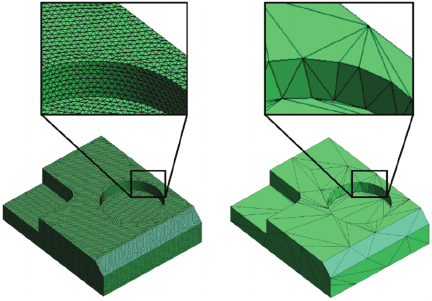 (a) Detailed mesh(b) Simplified mesh
Fig. 12. Mesh model.
6.2. Import of Simulation Data
First, the triangular mesh model data generated from the CAD data of the target object were imported. The two mesh models have different mesh sizes, as shown in Fig. 12. We defined the mesh model with a smaller mesh size as “detailed mesh,” and the one with a larger mesh size as “simplified mesh.” These were used to limit the calculation range and simplify the calculations. The size of the detailed mesh was set to be the same as the point distance per irradiation, which was determined by the measurement period and scanning speed. In addition, the detailed and simplified meshes corresponded geometrically, and several triangles of the detailed mesh were contained within each triangle of the simplified mesh.
Second, the characteristics of the laser probe and measurement conditions were imported for use in calculations.
6.3. Determination of Scanning Path
The scanning path generated by the CAT system is output as position \((x,y,z)\) in the CAD coordinate system, rotational angle (\(\mathit{rot}\)), and inclination angle (\(\mathit{inc}\)).
First, the measurement position was determined based on the start and end points. Therefore, a point cloud was generated by linear interpolation between the two points, considering the scanning speed. These points were saved as “measurement position.” The point clouds of the measurement position from the starting point to the end point were regarded as one scanning path. Subsequently, the generated scanning paths were saved individually as Path 2, Path 3, etc. In addition, the movement vector was defined as a normalized vector connecting the start and end points.
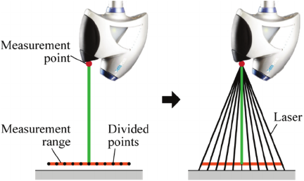
Fig. 13. Representation of laser.
Second, the direction of the laser incidence was determined using \(\mathit{rot}\) and \(\mathit{inc}\). When the angles are defined using Eqs. \(\eqref{eq:1}\) and \(\eqref{eq:2}\), the vector can be represented by normalizing Eq. \(\eqref{eq:3}\) 19. This was defined as the incident vector.
Finally, the measurement range was obtained by defining the normalized vector, which was orthogonal to both the movement and incident vectors. The normalized vector was defined as the range vector.
6.4. Calculation of Intersection
6.4.1. Linear Representation of Laser Light
Laser light was emitted from the tip of the probe and projected onto the surface of the object as a scanning line. The reflected laser light was detected by 1024 units of the light-receiving device. The laser light was regarded as 1024 lines emitted from the tip of the probe. Therefore, we represented the laser light as a group of straight lines using the characteristics of the probe. This representation is shown in Fig. 13. First, two points were generated at a distance of 93 mm from the measurement position along the incident vector at a distance of 20 mm and at a distance of \(-20\) mm along the range vector. The range between these two points is defined as the measurement range. Next, the point cloud divided the measurement range equally. The number of divisions was determined based on the mesh size and measurement density. Finally, a group of straight lines connecting the measurement point and divided points was generated.
6.4.2. Calculation
The intersection of the triangular mesh and the straight line representing the laser light was calculated. One line was extracted from the straight-line group. The intersection of the line and the simplified mesh model was calculated. If an intersection was not found, the calculation proceeded to the next line because the measured point did not exist for this line. If an intersection was found, we recalculated the intersection between the line and the detailed mesh contained within the triangle of the simplified mesh where the intersection was calculated. This calculation was applied only to the detailed mesh triangles within the target triangle. Therefore, calculations can be performed efficiently.
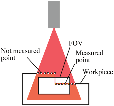
Fig. 14. Judgment of FOV inside or outside.
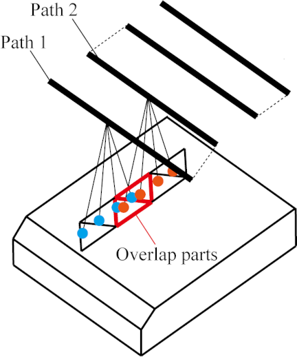
Fig. 15. Judgment of overlap.
6.4.3. Judgment of FOV Inside or Outside
Whether the intersection calculated in Section 6.4.2 within the FOV, is determined as follows. The rectangular area representing the FOV in the current measurement position was represented using the characteristics of the probe, as shown in Fig. 14. If an intersection did not exist in the range of a rectangular area, the point was not measured when measuring the target object. Therefore, the position of the intersection is not saved. Otherwise, it was saved. The processes in Sections 6.4.2 and 6.4.3 were performed in all groups of straight lines.
6.5. Judgment of Overlap
The overlap occurs when the measurement areas were duplicated. That is, the same parts were measured using multiple scanning paths. Therefore, we define the criterion for overlap occurrence as the number of times the same parts were measured by different paths. The target was a triangular mesh. By applying this criterion, the number of measurements for a single mesh with different paths can be regarded as the number of overlaps.
When the intersection is saved as described in Section 6.4.3, the path number used for the measurement is also saved for each mesh index containing the intersection. As a result, it is possible to judge the overlap occurrence quantitatively, as shown in Fig. 15, based on the number of times different paths are measured.
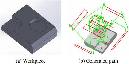
Fig. 16. Result of path generation.
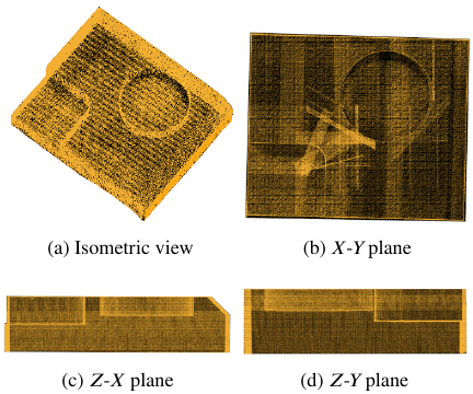
Fig. 17. Point cloud data.
6.6. Output of Result
If the count saved in Section 6.5 exceeds a certain threshold, the mesh is output as an overlapping occurrence part. The meshes are colored darker red according to the number of measurements. The meshes judged as overlapping parts are colored in blue. The centroid of the triangular meshes judged as an overlapping occurrence were output as the position of overlapped parts. When the generated path and the 1.5 mm detailed mesh were used, the overlap of all surfaces could be detected within 20 s. Through this overlap detection, information can be added to the measurement point cloud, indicating whether each point is near an overlapping part. Using this information, we could efficiently perform point-cloud reduction.
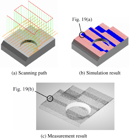
Fig. 18. Comparison between simulation result and measurement result.
7. Evaluation
7.1. Results of Measurement and Path Generation
A measurement was conducted using the scanning path generated by the CAT system. The target shape is shown in Fig. 16(a) and the generated scanning path is shown in Fig. 16(b). The point cloud data measured by the CMM are shown in Figs. 17(a) and (d). Consequently, the interference between the target object and the probe did not occur. In addition, no missing point-cloud regions were observed. However, an overlap occurred on part of the top surface. This overlap likely occurred because of excessive division of the scanning path to prevent missing point clouds. It was also found that the occurrence of overlaps caused by the generated path affected the density of the measured point cloud. Therefore, it is considered that the point cloud density can be adjusted by setting an appropriate path interval.
7.2. Results of Overlap Detection
This study conducted a comparative evaluation between the detection results of overlap by the simulator and the measured point cloud data. The simulation path is shown in Fig. 18(a), the detection result of the overlap is shown in Fig. 18(b), and the point cloud data are shown in Fig. 18(c). When the path shown in Fig. 18(a) was used, an overlap was detected within 3 s. An enlarged view of the overlap detection result is shown in Fig. 19(a), and the result of extracting the point cloud within the mesh size from the overlap coordinate values is shown in Fig. 19(b). The average width of the overlap coordinate values in Fig. 19(a) is 12.20 mm, whereas the width of the overlap point cloud in Fig. 19(b) is 13.18 mm. This difference is approximately 1 mm. Because the verification was conducted with a mesh size of 1.5 mm, this difference was unavoidable. Therefore, the detection results were considered sufficient. This error can be reduced by decreasing the mesh size. In addition, when the simulations were performed using the scanning paths generated for the side surfaces and other surfaces, results similar to those shown in Figs. 17(c) and 17(d) were obtained. Consequently, we confirmed that overlap regions were detected using the developed measurement simulator.
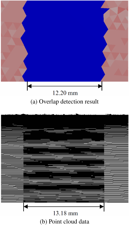
Fig. 19. Comparison of overlap regions.
8. Conclusion
This study developed a CAT system consisting of a path-generation system and a measurement simulator for a 3D measurement system using a line laser probe and a CMM. Using a path-generation system, a scanning path can be generated automatically to address the missing point clouds. Furthermore, by comparing the simulation results with the actual measurement results, sufficient agreement was found between the overlapping parts. Therefore, overlapping parts can be detected in advance using the proposed measurement simulation. Therefore, the proposed method can be applied to path generation based on the overlap detection results. Future work will focus on developing a method for point-cloud reduction based on the coordinates of overlapping parts.
- [1] T. Umehara, T. Ishida, K. Teramoto, and Y. Takeuchi, “Effective tool path generation method for roughing in multi-axis control machining,” Trans. of the Japan Society of Mechanical Engineers, Part C, Vol.73, No.732, pp. 2387-2393, 2007 (in Japanese). https://doi.org/10.1299/kikaic.73.2387
- [2] H. Kyogoku, “Recent trend on laser metal additive manufacturing,” J. of Japan Society of Precision Engineering, Vol.82, No.7, pp. 619-623, 2016 (in Japanese). https://doi.org/10.2493/jjspe.82.619
- [3] A. Matsubara, “Current status and trends of monitoring and control technology in machining process,” J. of the Society of Instrument and Control Engineers, Vol.41, No.11, pp. 781-786, 2002 (in Japanese). https://doi.org/10.11499/sicejl1962.41.781
- [4] R. Yamada, “Trend of quality assurance of steel products using machine vision systems,” Denki-seiko, Vol.79, No.4, pp. 313-318, 2008 (in Japanese). https://doi.org/10.4262/denkiseiko.79.313
- [5] O. Jusko, M. Neugebauer, H. Reimann, and R. Bernhardt, “Recent progress in CMM-based form measurement,” Int. J. Automation Technol., Vol.9, No.2, pp. 170-175, 2015. https://doi.org/10.20965/ijat.2015.p0170
- [6] S. Osawa, T. Takatsuji, and O. Sato, “High accuracy three-dimensional shape measurements for supporting manufacturing industries – Establishment of the traceability system and standardization –,” Synthesiology, Vol.2, No.2, pp. 101-112, 2009 (in Japanese). https://doi.org/10.5571/synth.2.101
- [7] M. Takezawa, K. Matsuo, and T. Ando, “Development of support system for ship-hull plate forming using laser scanner,” Int. J. Automation Technol., Vol.15, No.3, pp. 290-300, 2021. https://doi.org/10.20965/ijat.2021.p0290
- [8] T. Yoshizawa, “Recent trends in optical profilometry,” J. of the Society of Instrument and Control Engineers, Vol.50, No.2, pp. 80-88, 2011 (in Japanese). https://doi.org/10.11499/sicejl.50.80
- [9] PMT Technologies, “Measuring arm: Differences between contact and non-contact measurement methods,” 2025. https://www.pmt3d.com/measuring-arm-differences-between-contact-and-non-contact-measurement-methods/ [Accessed December 2, 2025]
- [10] Mitutoyo Europe. https://mitutoyo.eu/news/special-promotions/free-offline-programming-micat-planner [Accessed December 2, 2025]
- [11] L. Ding, S. Dai, and P. Mu, “CAD-based path planning for 3D laser scanning of complex surface,” Procedia Computer Science, Vol.92, pp. 526-535, 2016. https://doi.org/10.1016/j.procs.2016.07.378
- [12] N. D. M. Phan, Y. Quinsat, S. Lavernhe, and C. Lartigue, “Scanner path planning with the control of overlap for part inspection with an industrial robot,” The Int. J. of Advanced Manufacturing Technology, Vol.98, pp. 629-643, 2018. https://doi.org/10.1007/s00170-018-2336-8
- [13] K. Takenaka, “Construction of free form surface for reverse engineering,” J. of Japan Society for Design Engineering, Vol.32, No.12, pp. 454-457, 1997 (in Japanese).
- [14] K. Takasugi, N. Asakawa, and Y. Morimoto, “A surface parameter-based method for accurate and efficient tool path generation,” Int. J. Automation Technol., Vol.8, No.3, pp. 428-436, 2014. https://doi.org/10.20965/ijat.2014.p0428
- [15] ScienceDirect, “Diffuse reflection.” https://www.sciencedirect.com/topics/engineering/diffuse-reflection [Accessed December 2, 2025]
- [16] T. J. Fellers and M. W. Davidson, “Introduction to the Reflection of Light,” https://evidentscientific.com/en/microscope-resource/knowledge-hub/lightandcolor/reflectionintro [Accessed December 2, 2025]
- [17] Sensor Partners, “Triangulation measurement: how it works and what to use it for,” https://sensorpartners.com/en/knowledge-base/what-is-a-triangulation-or-triangulation/ [Accessed December 2, 2025]
- [18] A. Isheil, J.-P. Gonnet, D. Joannic, and J.-F. Fontaine, “Systematic error correction of a 3D laser scanning measurement device,” Optics and Lasers in Engineering, Vol.49, No.1, pp. 16-24, 2011. https://doi.org/10.1016/j.optlaseng.2010.09.006
- [19] E. W. Weisstein, “Rotation Matrix,” MathWorld–A Wolfram Resource. https://mathworld.wolfram.com/RotationMatrix.html [Accessed December 2, 2025]
This article is published under a Creative Commons Attribution-NoDerivatives 4.0 Internationa License.