Research Paper:
Investigating an Integrated Scheduling Model for Steel Manufacturing Under Uncertainty
Daisuke Morita*,† and Haruhiko Suwa**
*Department of Electrical and Electronic Systems Engineering, Osaka Metropolitan University
1-1 Gakuencho, Naka-ku, Sakai, Osaka 599-8531, Japan
†Corresponding author
**Department of Mechanical Engineering, Setsunan University
Neyagawa, Japan

Steel manufacturing involves complex scheduling because of the interdependence between the steelmaking and rolling processes. This study proposes an integrated scheduling model for long-term planning of these processes under uncertainty. The proposed model abstracts an existing detailed scheduling model using two key techniques: charge integration and rolling process simplification. Through numerical experiments, we evaluated the characteristics and effectiveness of the model under different objective functions and time and resource buffer allocation strategies. The results demonstrate that the model achieves computational efficiency while maintaining accuracy.
1. Introduction
In steel manufacturing, as illustrated in Fig. 1, the final steel product is produced via two distinct processes: steelmaking and rolling 1,2. The steelmaking process comprises three main stages. First, molten pig iron is refined in a basic oxygen furnace (BOF) to yield molten steel. The molten steel is then transported to the refining stage in single-ladle units, each called a “charge.” During the refining stage, impurities are further eliminated and the composition of the molten steel is adjusted. Subsequently, continuous casting processes multiple charges from the same group, referred to as a “cast,” to produce semi-finished products. This process solidifies molten steel into slabs, blooms, and billets in a continuous and efficient manner. Finally, during the rolling process, these semi-finished products are shaped into final steel products via hot and cold rolling. The entire process must satisfy the necessary specifications while ensuring timely delivery.
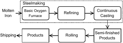
Fig. 1. Steel manufacturing process.
To produce steel efficiently, it is crucial to develop a schedule for the steelmaking and rolling processes that considers the complex constraints related to machine assignments, casting sequences, transportation times, and the availability of semi-finished products. Although several scheduling methods have been proposed for steelmaking process 3,4,5 and rolling process 6,7, most existing studies have concentrated on detailed scheduling models that focus on only one of these processes. However, as steelmaking and rolling processes are interdependent, the outcomes of the steelmaking process can influence the operation of the rolling process. A recent review identified integrated scheduling models that simultaneously handle steelmaking and rolling processes as important research directions 8.
Integrated models are particularly important when uncertainty is taken into account, such as variability in processing times, machine breakdowns, and unexpected disruptions. These uncertainties may lead to delays in steelmaking operations that can propagate through the processes and ultimately result in delays in the delivery of the final product. Although some studies have proposed integrated models 9,10, they did not explicitly account for the uncertainties that cause operational delays. Furthermore, these studies adopted detailed scheduling models that determine the start times of operations at each machine, which can restrict the tractable problem size and reduce the applicability to long-term planning.
The above discussion reveals a critical gap: a lack of integrated scheduling models that are computationally efficient for long-term planning. Excessive abstraction can remove characteristic scheduling behaviors such as the sensitivity of generated schedules to the selected objective function, delays caused by uncertainty, and their absorption by buffers, which we refer to as a reduction in accuracy. Our previous work aimed to address this gap by defining an integrated scheduling model and exploring buffer-based countermeasures 11,12. In this study, buffer refers to the time or resource slack allocated to a schedule to absorb delays. Through numerical experiments, we confirmed that buffer allocation mitigates the impact of delays and uncertainties, thereby enhancing the schedule robustness. However, this model does not sufficiently analyze its consistency with detailed scheduling models. This consistency is crucial in production environments, where multiple schedules of different granularities must be managed to align long-term strategic plans with detailed schedules.
Based on the above analysis, we addressed the following research questions:
-
RQ1:
How can we construct an integrated scheduling model for the long-term planning of both steelmaking and rolling processes that maintains consistency with a detailed schedule?
-
RQ2:
Does the constructed integrated model possess sufficient accuracy to capture schedule variations caused by the objective function selection, delay propagation during execution, and buffer absorption effects?
To address RQ1, we abstracted a detailed model using two key techniques: charge integration and rolling process simplification. For long-term planning while maintaining consistency with detailed scheduling models, this model uses two key abstraction techniques: charge integration and simplification of the rolling process. In the steelmaking process, we identify multiple charges belonging to simultaneous casts and combine them into an integrated job comprising operations at each stage. Each operation in the integrated job represents the collective processing of the consolidated charges at each stage. As the steelmaking process is generally a bottleneck 13, the rolling process is significantly simplified. Specifically, we focus only on determining the start time of the first rolling operation, ensuring that it satisfies the deadline derived from backward scheduling. The model also accounts for uncertainty by assuming that processing times may be delayed during execution, and a buffer allocation framework is incorporated as a countermeasure. To generate the schedule, we formulated the problem for a constraint programming (CP) solver, which is generally well-suited for scheduling problems owing to its efficient tree search based on constraint propagation.
To address RQ2, numerical experiments were conducted to validate the accuracy of the model in capturing schedule variations. In these experiments, delay simulations were performed to analyze the characteristics of the target model. The problem instances were generated based on detailed scheduling instances from previous literature. In the delay simulation, we examined variations in the simulation results caused by objective function selection, delay propagation during execution, and buffer absorption effects. The experimental results demonstrate that the proposed model effectively captures these schedule variations while maintaining an appropriate level of abstraction.
This study makes the following contributions:
-
We propose a computationally efficient integrated scheduling model for long-term planning of both steelmaking and rolling processes that maintains consistency with detailed scheduling models. By abstracting the detailed model through charge integration and simplifying of the rolling process, our model can generate schedules for long-term planning horizons with low computational costs while preserving essential operational constraints. This directly addresses RQ1.
-
The accuracy of the proposed model is validated through numerical experiments. The results of the delay simulations demonstrate that our model can appropriately capture schedule variations caused by objective function selection, delay propagation during execution, and buffer absorption effects. This confirms that the model is sufficiently accurate for evaluating different scheduling strategies under uncertainty, thereby addressing RQ2.
2. Model Construction
2.1. Integrated Model Overview and Abstraction Techniques
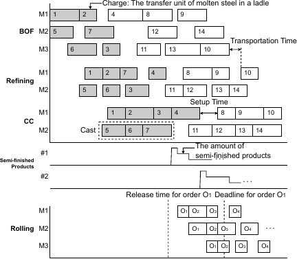
Fig. 2. A scheduling model for the steelmaking and rolling processes.
We constructed an integrated model based on the detailed scheduling model illustrated in Fig. 2, which refers to the steelmaking process described in a previous study 8. We employed a detailed scheduling model to construct an integrated model. This model is an extension of the flexible-flow shop scheduling problem 14,15. Each operation represents the start and finish times of the charges at each stage, including BOF, refining, and continuous casting (CC).
The key constraints include the range of transportation times between the stages, casting requirements, and setup times between the casts. The transportation time constraint ensures that processing of a charge at the next stage begins within the range \([\Delta^{\min},\Delta^{\max}]\) after finishing the previous stage. The minimum transportation time \(\Delta^{\min}\) denotes the time required to move a charge to the next stage. The maximum transportation time \(\Delta^{\max}\) represents the time limit imposed to prevent quality degradation caused by the temperature drop of the charge. The casting requirements mandate that all charges belonging to the same cast must be processed consecutively, thereby ensuring no interruptions in processing. A setup time is required between consecutively processed casts on the same machine. Operations in the rolling process, referred to as orders, utilize semi-finished products produced in the steelmaking process. Each order must be processed on all designated machines by its deadline.
In the steelmaking process, charges processed concurrently in the continuous casting stage are generally processed during the same time periods as those in the other stages. Therefore, as shown in Fig. 3, we identify these charges and consolidate their processes into single operations at each stage. We refer to this collection of operations across all the stages as integrated jobs. The operation of job \(j\) in stage \(k\) is denoted by \(J_{jk}\). This abstraction is expected to achieve computational efficiency, enabling feasible solutions to be found within a reasonable time, even for planning periods of approximately one week.
For these integrated jobs, the time gap between the completion of an operation at stage \(k-1\) and its subsequent completion at stage \(k\) is constrained. This constraint is necessary to ensure that the proposed model still respects the minimum and maximum transportation time range \([\Delta^{\min},\Delta^{\max}]\) between the charges in the detailed model. This gap, denoted \([\tau^{\min}_k, \tau^{\max}_k]\), is derived from the minimum/maximum transportation time and charge processing time in the detailed model. This is defined as follows:
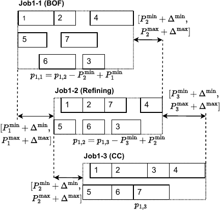
Fig. 3. Integration of gray-shaded charges illustrated in Fig. 2.
To maintain consistency with the transportation time constraints, while ensuring that the integrated jobs have appropriate processing times, we define the processing time \(p_{jk}\) of job \(j\) in stage \(k\) as follows:
In the integrated model, the amount of semi-finished products from a completed job equals the sum of the semi-finished products from all consolidated charges. In addition, one stage cannot process multiple jobs simultaneously.
During the rolling process in the detailed scheduling model, the start time of each order must be determined between its release time and deadline. To simplify the problem, we convert this scheduling problem into one in which only the start time of the first operation must be determined. This first operation must meet its start-time deadline, which is calculated through backward scheduling from the original order deadline. Fig. 4 presents a scheduling example of the model.
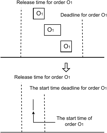
Fig. 4. Transformation of rolling scheduling into a start time decision problem.
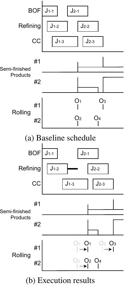
Fig. 5. Comparison of the baseline schedule and execution results (each number in the order rows indicates which semi-finished product is consumed by the order).
The proposed integrated scheduling model must satisfy several key constraints: time gaps between consecutive stages, exclusive processing of jobs at each stage, inventory constraints for semi-finished products, and release times and deadlines for orders. A feasible schedule that satisfies all these constraints, referred to as the baseline schedule, is shown in Fig. 5(a).
2.2. Delay Propagation and Buffer Allocation Strategies
Although the steel manufacturing industry follows a baseline schedule, delays can occur during the execution phase. Because time gap constraints exist between job operations in the steelmaking process, a delay in completing a job operation at an earlier stage caused by machine failures, extended processing times for charges, or other factors will also postpone the start of subsequent job operations (Fig. 5(b)). Propagation of delays can result in deadline violations. To mitigate such delays, this study considers two types of buffer allocation strategies.
Buffers were incorporated into the baseline schedule to reduce delays that may occur during execution. This study analyzed the impact of two types of buffers: time and resource buffers.
A time buffer is slack time intentionally added to the baseline schedule to absorb delays. This approach is widely used in project scheduling, especially in critical chain project management methodologies 16,17. In the target problem, a time buffer was inserted by postponing the start time of the order during the rolling process. Time buffer allocation can be viewed as delaying the start time of an order during the scheduling phase, as shown in Fig. 5(b). As time buffers can absorb delays that occur during the steelmaking process, this approach enhances schedule predictability.
A resource buffer is an extra stock of semi-finished products generated in the steelmaking process 18,19. When job operations are delayed, the production of semi-finished products is also delayed, which affects their availability for the rolling process, leading to a delay in the order start time. In such cases, the resource buffers can mitigate the impact of these delays, as shown in Fig. 6.
In this study, a resource buffer was implemented by increasing the production of semi-finished products from jobs. However, we limited the quantity and types of the additional semi-finished products to reflect realistic production conditions. Numerical experiments discussed the specifics of these limitations.
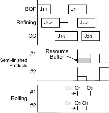
Fig. 6. Delay absorption by resource buffer.
3. Mathematical Formulation
3.1. Problem Formulation and Constraints
We formulated a scheduling problem based on the model described in the previous section. The formulation employed logical expressions compatible with the CP solver used to solve the target problem in this study 20,21. The notations used for the target problem are listed in Table 1.
We consider three types of objective functions: minimizing the makespan, maximizing the total earliness, and maximizing the minimum earliness, as defined below.
The second term in the objective function defined in Eqs. (3) and (4) accounts for the maximum delay beyond the deadline, and imposes penalties for deadline violations. Instead of enforcing deadline constraints directly, we incorporate them as penalty terms in the objective function. This setting prevents the search from stagnating when feasible solutions are difficult to find while guiding it toward solutions that minimize tardiness. The parameter \(\lambda\) is set to a sufficiently large value (e.g., as an upper bound of the objective function value) to prioritize avoiding deadline violations. In numerical experiments, this setting enabled the early discovery of schedules without deadline violations. Conversely, Eq. (5) does not require an explicit penalty for deadline violations.
Table 1. Notation.

Table 2. Experimental conditions.

The constraints of the target problem are as follows:
3.2. Execution Procedure
The execution result of the baseline schedule is calculated through the following procedure:
-
Initialize current time \(t \leftarrow 0\).
-
Identify all job operations \(J_{jk}\) and orders \(O_i\) that are scheduled to start at time \(t\), i.e., satisfying \(s^\text{J}_{jk} = t\) and \(s^\text{O}_i = t\).
-
The identified operations and orders are executed and the actual processing times of the job operations are obtained, which may differ from the planned processing times owing to delays.
-
If any constraint is violated owing to the updated actual processing times, reschedule the start times for all unstarted job operations and orders according to the following rules:
-
Schedule orders and job operations to start as early as possible, while ensuring that all constraints are satisfied.
-
When multiple job operations or orders can start simultaneously, prioritize those with earlier originally planned start times. In the case of ties, select the job or order with the smaller index.
-
-
Increment \(t\) by one and return to Step 2 until all job operations and orders are completed.
3.3. Buffer Allocation Procedure
Time buffer allocation: When allocating time buffers, we maintain the start times of all job operations in a fixed baseline schedule. For each order \(O_i\), the start time \(s^\text{O}_i\) is delayed by up to the specified buffer size \(B^\textrm{T}_i\), while ensuring that the deadline constraint is not violated. Specifically, the start time \(s^\text{O}_i\) was adjusted as follows:
Resource buffer allocation: For resource buffer allocation, we determined both the quantity and type of resource buffers to be allocated. In the baseline schedule, resource buffers are allocated to jobs in ascending order of their start times. For each job \(j\) and semi-finished product type \(\ell\), we allocate the resource buffers according to
4. Numerical Experiments
In numerical experiments, we analyzed the characteristics of the target model. Specifically, we examined how the settings of the objective function, along with the allocation of resource and time buffers, influence the simulation results.
We generated 100 problem instances based on the conditions specified in Table 2, where \(U[a,b]\) represent random variables that follow a uniform distribution over the intervals \([a,b]\). The parameters related to the steelmaking process were based on 1. The steelmaking process in our model consisted of three stages: BOF, refining, and CC. The number of semi-finished product types was set to \(N^\text{R} = 8\), and the scheduling period was defined as 10,080 min, corresponding to one week.
Based on the existing literature, we specified the number of charges per job, range of charge processing times at each stage, transportation time between stages, and setup time between casts. Processing time can vary even for the same steel grade owing to the chemical composition determined at the blast-furnace stage and the operating conditions at each stage. Therefore, we modeled the processing time as a random variable drawn from a uniform distribution. It is assumed that two continuous casting machines were available and that each job produced two types of semi-finished products selected from the eight available types. The production volume of the secondary type \(a^\text{J}_{j\ell_{j2}}\) was determined based on the assumption that the numbers of charges in the two casts combined in a job were similar. To provide sufficient scheduling flexibility, the release time and deadline for each order were set to half a day before and after the planned start day, respectively.
The number of jobs was maximized, subject to the constraint that the total processing and setup times did not exceed the scheduling period. Similarly, the number of orders was maximized subject to the constraint that the consumption of semi-finished products did not exceed the quantity produced by the jobs. Consequently, the number of jobs and orders varies depending on the specific problem instance. The details of the instance-generation procedure are provided in Appendix B.
First, we examine the influence of the objective function on the simulation results. For each problem instance, a schedule was generated using the CP Optimizer 22 based on the formulation described in Section 3. The objective functions were as follows:
-
Minimizing makespan (Eq. (3)),
-
Maximizing total earliness (Eq. (4)),
-
Maximizing minimum earliness (Eq. (5)).
The model was implemented using IBM ILOG CP Optimizer v22.1.1.0. A time limit of 300 s was applied to each solution, and all other parameters were maintained at their default settings. Feasible schedules were successfully generated for all problem instances within this time limit. Fig. 7 presents a Gantt chart of the baseline schedule.
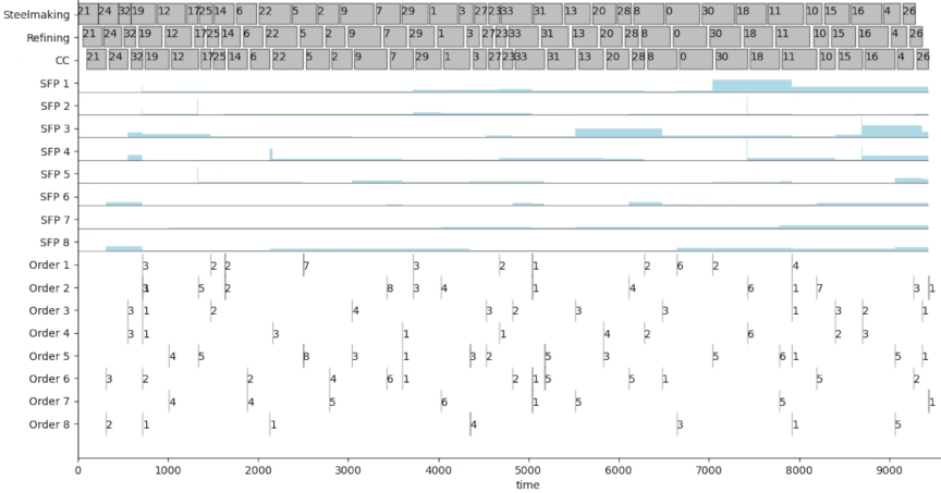
Fig. 7. Baseline schedule for steelmaking, semi-finished products, and orders (the number illustrated in each order indicates the number of orders starting at the same time).
Table 3. Comparison of evaluation metrics for different objective functions.

A delay simulation was performed on the baseline schedules, following the procedure described in the previous section. During the simulation, the job processing times experienced delays. In the simulation, the realized processing time is known at the start of each job. The delay amounts follow the distribution \(U[0, \alpha p_{jk}]\), where \(\alpha=0.10,0.15,0.20\). For each combination of problem instance, objective function, and delay parameter \(\alpha\), 100 simulations were conducted.
Table 3 presents two evaluation metrics: the average number of orders past the deadline (#Tard) and the average deviation between planned and actual order start times (Deviation) for each objective function. Table 3 lists the performance differences based on objective functions. Maximizing total earliness reduces deviations in the order start times. With this objective, there is a tendency to schedule many orders in earlier time slots. These orders are less affected by delays because delays tend to accumulate later in the schedule. Maximizing minimum earliness reduces delayed orders by preventing orders from starting close to their deadline.
Next, a simulation was conducted by applying two types of buffers—resource buffers (size \(=\) 1, 2, 3) and time buffers (size \(=\) 60, 120, 180)—to the schedule optimized for minimum earliness (Eq. (5)). We impose limitations on the resource buffer allocation. Specifically, we can only increase production volume \(a^\text{J}_{j\ell_{j2}}\) by 200 for jobs in which production volume \(a^\text{J}_{j\ell_{j2}}\) is smaller than \(a^\text{J}_{j\ell_{j1}}\). In addition, the buffer size determines the maximum number of jobs for which resource buffers can be allocated for each semi-finished product type. The results are summarized in Table 4. The problem instances, delay parameter \(\alpha\), and evaluation metrics used in this experiment were the same as in Table 3.
The results illustrate the effectiveness of buffer allocation and highlight the different characteristics of the two buffer types. Allocating time buffers effectively reduces the deviations in the start times of orders. Thus, the time buffer approach is useful for enhancing the schedule predictability in the rolling process. However, since this approach essentially delays the start time of the order, its contribution to reducing delivery delays (#Tard) is limited. By contrast, resource buffer allocation effectively reduces delivery delays. Although resource buffers also improve schedule predictability in the rolling process, their impact is less significant than that of time buffers.
Table 4. Comparison of evaluation metrics for different buffer allocations.

5. Discussion
5.1. Research Question Analysis
Numerical experiments provide evidence supporting the effectiveness of our proposed integrated scheduling model under the tested conditions. The results demonstrate that the model achieves a balance between computational efficiency and scheduling accuracy, suggesting its potential suitability for long-term planning in steel manufacturing under uncertainty. Based on the numerical experiments, we address the research questions posed in Section 1.
RQ1 analysis: We construct an integrated scheduling model that maintains consistency with detailed scheduling using two key abstraction techniques:
-
Charge integration: Multiple charges processed simultaneously in continuous casting were consolidated into an integrated job while preserving the transportation time constraints, which ensure consistency with the detailed model’s charge-level constraints.
-
Rolling process simplification: The rolling scheduling was simplified to focus on determining the start time of the first operation using backward scheduling from the original deadline, ensuring that the deadline constraints remained consistent with the detailed model.
These abstraction techniques maintain the essential operational constraints of the detailed model, while achieving computational efficiency.
RQ2 analysis: The experimental results confirm that the integrated model is sufficiently accurate in capturing schedule variations caused by the three factors specified in RQ2.
-
Objective function selection: The model demonstrates distinct schedule variations based on different objective functions. Total earliness maximization reduces start time deviations, whereas minimum earliness maximization minimizes deadline violations. These differentiated performance patterns indicate that the model accurately captures schedule variations resulting from the objective function selection and can support different operational priorities in steel manufacturing.
-
Delay propagation during execution: The simulation results show realistic delay propagation behavior, with increasing delay rates leading to proportional increases in both deadline violations and schedule deviations. This demonstrates that the model accurately captures schedule variations.
-
Buffer absorption effects: Both time and resource buffers demonstrated measurable effectiveness in mitigating delays, with distinct characteristics. Time buffers primarily enhance schedule predictability by reducing deviations in the order start times, whereas resource buffers are more effective at preventing deadline violations. This differentiation confirms that the model accurately captures schedule variations resulting from the buffer absorption effects.
5.2. Limitations and Future Directions
This study has several limitations that should be acknowledged. First, the experimental conditions employed simplified parameters and settings, rather than a comprehensive real-world representation. The delay simulation assumes uniform delay distributions across all operations, and does not account for the complex interdependencies between the different types of manufacturing disruptions that may occur in actual steel production environments. In addition, the buffer allocation strategies are implemented using simplified rules, which may not capture the full complexity of resource management decisions in practice. These simplifications were designed to enable a systematic evaluation of the fundamental characteristics of the proposed model.
Future studies should address these limitations by incorporating more realistic constraints and conditions to improve the practical applicability of the model to actual steel manufacturing environments. Specifically, future research should include: (1) more sophisticated delay models that reflect the stochastic nature of real manufacturing processes, (2) validation using actual production data from steel plants, and (3) an extension of the buffer allocation framework.
6. Conclusion
This study proposes an integrated model for steel manufacturing scheduling under uncertainty by addressing two research questions. Regarding RQ1, we demonstrated that the integrated model maintains consistency with detailed scheduling through charge integration and rolling process simplification, while achieving computational efficiency. For RQ2, the numerical experiments confirmed that the model accurately captured schedule variations caused by objective function selection, delay propagation during execution, and buffer absorption effects. These findings demonstrate that the proposed model provides sufficient accuracy for evaluating different scheduling strategies under uncertainty, while maintaining computational tractability for long-term planning applications.
Future work will incorporate more realistic manufacturing conditions and parameter settings that reflect actual steel production and validate the practical applicability of the model in real-world operations. We also identified and analyzed the conditions under which the formulations may become inconsistent.
7. Appendix A. CP Model Construction
This study constructs the scheduling model defined by Eqs. (3)–(13) using the variables and functions provided by the IBM ILOG CP Optimizer. Definitions of the variables and functions, together with the objective functions and constraints formulated using them, are as follows.
7.1. Decision Variables
7.1.1. Interval Variables
In the CP Optimizer, interval variables are used to model activities characterized by a start time, end time, and fixed size. In this study, we introduce interval variables to represent integrated jobs and orders.
-
Interval variable \(t^{\mathrm{J}}_{jk}\) represents the operation of integrated job \(j \in \mathcal{J}\) at stage \(k \in \mathcal{M}\) and has fixed size \(p_{jk}\).
-
Interval variable \(t^{\mathrm{O}}_{i}\) represents order \(i \in \mathcal{O}\) and has zero duration.
7.1.2. Sequence Variables
Sequence variable \(\sigma_k\) represents the processing sequence of integrated jobs at stage \(k \in \mathcal{M}\).
7.1.3. Modeling Functions
-
\(\mathop{\mathrm{start}}(t)\): the start time of interval variable \(t\).
-
\(\mathop{\mathrm{end}}(t)\): the end time of interval variable \(t\).
-
\(\mathop{\mathrm{no\_overlap}}(\sigma, S)\): a constraint ensuring that the interval variables in sequence variable \(\sigma\) do not overlap in time and that the minimum setup times \(S\) between consecutive intervals are respected.
-
\(\mathop{\mathrm{same\_sequence}}(\sigma_1, \sigma_2)\): a constraint enforcing identical orderings of interval variables in the two sequence variables \(\sigma_1\) and \(\sigma_2\).
-
\(\mathop{\mathrm{step\_at\_start}}(t, a)\): a step function that increases the cumulative quantity by \(a\) at the start time of interval variable \(t\).
-
\(\mathop{\mathrm{step\_at\_end}}(t, a)\): a step function that increases the cumulative quantity by \(a\) at the end time of interval variable \(t\).
7.2. Objective Functions and Constraints
Using the above variables and functions, the objective functions and constraints can be expressed as follows:
7.2.1. Objective Functions
7.2.2. Constraints
8. Appendix B. Problem Instance Generation
8.1. Generate Integrated Jobs
The processing time and production quantities of integrated job \(j\) are determined as follows.
-
Determine integrated processing times.
The processing time for Stage 3 (CC) is calculated as
\begin{align*} p_{j}^{3} = n_j \cdot U[35,45]. \end{align*}The processing times for the refining and BOF stages were calculated using Eq. (2) as\begin{align*} p_{j,2} &= p_{j,3} - (35+10) + (30+10) = p_{j,3} - 5,\\ p_{j,1} &= p_{j,2} - (30+10) + (45+10) = p_{j,2} + 15. \end{align*} -
Assign the quantities of semi-finished product.
Randomly select two distinct semi-finished product types \(\ell_1 \neq \ell_2\) and set
\begin{align*} &a_{\ell_1} = 200 \cdot n_j, \\ &a_{\ell_2} = 200 \cdot \max\left(n_j - U[0,2], 3\right). \end{align*} -
Check weekly load and iterate.
If the total CC-stage processing time and cast setup time of the integrated jobs generated so far do not exceed the one-week horizon (10,080 min), add integrated job \(j\) to job set \(\mathcal{J}\). Otherwise, terminate the procedure.
8.2. Generate Orders in the Rolling Process
The quantities of semi-finished products, release times, and due dates of order \(i\) are determined as follows:
-
Compute semi-finished product inventories.
The produced quantities \(a^J_{i\ell}\) of all the integrated jobs for each semi-finished product type \(\ell\) were summed to obtain the initial inventory of each type.
-
Select a semi-finished product.
Randomly select a semi-finished product type \(\ell\) whose remaining inventory is nonzero. If no such product type exists, terminate the procedure.
-
Generate demands sequentially.
Draw the consumption quantity \(q \sim U[50,500]\). If the remaining inventory of \(\ell\) is less than \(q\), truncate \(q\) to the available amount. Then decrease the inventory of \(\ell\) by \(q\).
-
Set release times and due dates.
Draw a planned starting day \(\mathrm{day}_i \sim U[1,7]\), and calculate the release time and due date. Then, add order \(i\) to order set \(\mathcal{O}\).
- [1] J. Hong, K. Moon, K. Lee, K. Lee, and M. L. Pinedo, “An iterated greedy matheuristic for scheduling in steelmaking-continuous casting process,” Int. J. of Production Research, Vol.60, No.2, pp. 623-643, 2022. https://doi.org/10.1080/00207543.2021.1975839
- [2] S. K. Dutta and Y. B. Chokshi, “Basic concepts of iron and steel making,” Springer Nature, 2020. https://doi.org/10.1007/978-981-15-2437-0
- [3] Q.-K. Pan, “An effective co-evolutionary artificial bee colony algorithm for steelmaking-continuous casting scheduling,” European J. of Operational Research, Vol.250, No.3, pp. 702-714, 2016. https://doi.org/10.1016/j.ejor.2015.10.007
- [4] J. Long, Z. Sun, P. M. Pardalos, Y. Bai, S. Zhang, and C. Li, “A robust dynamic scheduling approach based on release time series forecasting for the steelmaking-continuous casting production,” Applied Soft Computing, Vol.92, Article No.106271, 2020. https://doi.org/10.1016/j.asoc.2020.106271
- [5] Z. Xu, Z. Zheng, and X. Gao, “Energy-efficient steelmaking-continuous casting scheduling problem with temperature constraints and its solution using a multi-objective hybrid genetic algorithm with local search,” Applied Soft Computing, Vol.95, Article No.106554, 2020. https://doi.org/10.1016/j.asoc.2020.106554
- [6] L.-L. Liu, X. Wan, Z. Gao, X. Li, and B. Feng, “Research on modelling and optimization of hot rolling scheduling,” J. of Ambient Intelligence and Humanized Computing, Vol.10, pp. 1201-1216, 2019. https://doi.org/10.1007/s12652-018-0944-7
- [7] Q.-K. Pan, L. Gao, and L. Wang, “A multi-objective hot-rolling scheduling problem in the compact strip production,” Applied Mathematical Modelling, Vol.73, pp. 327-348, 2019. https://doi.org/10.1016/j.apm.2019.04.006
- [8] M. Lee, K. Moon, K. Lee, J. Hong, and M. Pinedo, “A critical review of planning and scheduling in steel-making and continuous casting in the steel industry,” J. of the Operational Research Society, Vol.75, No.8, pp. 1421-1455, 2024. https://doi.org/10.1080/01605682.2023.2265416
- [9] Y. Tan, M. Zhou, Y. Wang, X. Guo, and L. Qi, “A hybrid MIP–CP approach to multistage scheduling problem in continuous casting and hot-rolling processes,” IEEE Trans. on Automation Science and Engineering, Vol.16, No.4, pp. 1860-1869, 2019. https://doi.org/10.1109/TASE.2019.2894093
- [10] C. Xu, G. Sand, I. Harjunkoski, and S. Engell, “A new heuristic for plant-wide schedule coordination problems: The intersection coordination heuristic,” Computers & Chemical Engineering, Vol.42, pp. 152-167, 2012. https://doi.org/10.1016/j.compchemeng.2011.12.014
- [11] D. Morita and H. Suwa, “A buffer-based steel production scheduling under uncertain environment,” Proc. of the 2024 Int. Symp. on Flexible Automation, Article No.V001T05A001, 2024. https://doi.org/10.1115/ISFA2024-130573
- [12] H. Suwa and D. Morita, “Optimization model for resource-buffer scheduling toward resilient steel production,” Tetsu-to-Hagané, Vol.110, No.14, pp. 1034-1042, 2024 (in Japanese). https://doi.org/10.2355/tetsutohagane.TETSU-2024-041
- [13] L. Tang, P. B. Luh, J. Liu, and L. Fang, “Steel-making process scheduling using Lagrangian relaxation,” Int. J. of Production Research, Vol.40, No.1, pp. 55-70, 2002. https://doi.org/10.1080/00207540110073000
- [14] R. Ruiz, F. S. Şerifoğlu, and T. Urlings, “Modeling realistic hybrid flexible flowshop scheduling problems,” Computers & Operations Research, Vol.35, No.4, pp. 1151-1175, 2008. https://doi.org/10.1016/j.cor.2006.07.014
- [15] B. Naderi, S. Gohari, and M. Yazdani, “Hybrid flexible flowshop problems: Models and solution methods,” Applied Mathematical Modelling, Vol.38, No.24, pp. 5767-5780, 2014. https://doi.org/10.1016/j.apm.2014.04.012
- [16] L. P. Leach, “Critical Chain Project Management,” Artech House, 2014.
- [17] D. Morita and H. Suwa, “An optimization method for critical chain scheduling toward project greenality,” Int. J. Automation Technol., Vol.6, No.3, pp. 331-337, 2012. https://doi.org/10.20965/ijat.2012.p0331
- [18] O. Lambrechts, E. Demeulemeester, and W. Herroelen, “Proactive and reactive strategies for resource-constrained project scheduling with uncertain resource availabilities,” J. of Scheduling, Vol.11, No.2, pp. 121-136, 2008. https://doi.org/10.1007/s10951-007-0021-0
- [19] M. Shariatmadari and N. Nahavandi, “A new resource buffer insertion approach for proactive resource investment problem,” Computers & Industrial Engineering, Vol.146, Article No.106582, 2020. https://doi.org/10.1016/j.cie.2020.106582
- [20] L. Meng, C. Zhang, Y. Ren, B. Zhang, and C. Lv, “Mixed-integer linear programming and constraint programming formulations for solving distributed flexible job shop scheduling problem,” Computers & Industrial Engineering, Vol.142, Article No.106347, 2020. https://doi.org/10.1016/j.cie.2020.106347
- [21] P. Baptiste, C. Pape, and W. Nuijten, “Constraint-Based Scheduling: Applying Constraint Programming to Scheduling Problems,” Springer, 2001. https://doi.org/10.1007/978-1-4615-1479-4
- [22] P. Laborie, J. Rogerie, P. Shaw, and P. Vilím, “IBM ILOG CP optimizer for scheduling: 20+ years of scheduling with constraints at IBM/ILOG,” Constraints, Vol.23, pp. 210-250, 2018. https://doi.org/10.1007/s10601-018-9281-x
This article is published under a Creative Commons Attribution-NoDerivatives 4.0 Internationa License.