Research Paper:
Improving Efficiency Through Data Selection for Remote Injection Molding Condition Monitoring Systems Using the Mahalanobis–Taguchi Method
Keigo Kudo†, Yuta Abe, Makoto Fukushima, Yoshio Fukushima, and Naoki Kawada
Graduate School of Engineering, Saitama Institute of Technology
1690 Fusaiji, Fukaya, Saitama 369-0293, Japan
†Corresponding author

Injection molding is the most common method for manufacturing plastic products. However, products made by injection molding often exhibit various molding defects. One major contributing factor to these defects is mold temperature, especially at the cavity section where the resin enters. In our laboratory’s research, the feasibility of measuring the cavity temperature using non-contact thermometers by making simple modifications around the mold cavity area was investigated. It was also examined whether it is possible to distinguish between normal and defective molded products—specifically those with short shots—based on this temperature data. Analyzing data from predefined temperature measurement points raises concerns about significantly increased computation times. For remote monitoring applications, it is necessary to reduce the number of measurement points to decrease data volume. In this paper, an attempt is made to reduce the number of measurement points used in analysis by selecting items with an orthogonal array. As a result, the number of measurement points for analysis was reduced by 55%, thereby decreasing computation time and achieving favorable results for implementing a remote monitoring system equipped with defect detection functionality, which is reported here.
1. Introduction
In the coming years, the ongoing demographic shift toward a declining birth rate and an aging population is expected to cause a serious shortage of next-generation workers, potentially disrupting the transfer of technological expertise. Even if the Japanese government’s aggressive measures to address the demographic crisis yield positive results, their full implementation will likely require significant time. Consequently, the current manufacturing environment faces a critical issue: insufficient time to ensure knowledge transfer and workforce sustainability 1,2. In response, research on manufacturing support systems that integrate various sensors, IT devices, and artificial intelligence (AI) technologies has gained considerable momentum 3,4,5,6,7,8,9,10,11. The applications of condition-monitoring techniques, particularly in machine tools and related fields, are being actively investigated and evaluated for effectiveness. In addition, inspection systems using AI algorithms to classify products as acceptable or defective have attracted increasing attention. Thus, AI-enabled condition monitoring systems are expected to play a pivotal role in supporting future manufacturing sites. This study focused on remote condition-monitoring systems in plastic injection molding. Plastic products are generally produced through injection molding, a process in which various factors can lead to defects. One common defect is the “short shot 12,” which occurs when the resin fails to fill the mold cavity completely due to factors such as insufficient resin or mold temperature, or low injection pressure. Short shots can also result from air trapped in complex mold geometries, impeding resin flow; however, resin and mold temperatures are considered to have a particularly strong influence. Therefore, we hypothesized that more accurate condition monitoring could be achieved by observing the temperature near the mold surface where the product is formed. Molding defects caused by surface temperature include not only short shots, but also warpage and burn marks. However, in this experiment, the focus was on short shots, which can be easily induced. The objective of this study was to construct a remote condition-monitoring system that uses data obtained from a non-contact thermometer (infrared thermal camera). For data analysis, we applied the Mahalanobis–Taguchi (MT) method, a pattern recognition technique 13,14,15,16,17,18. The objectives of this study are as follows: (1) to confirm the feasibility and performance of detecting molding defects, particularly short shots; (2) to examine methods for selecting optimal measurement data to improve detection performance; and (3) to investigate the relationship between the selected data and the mold structure.
In the future, we aim to propose a low-cost condition-monitoring system that minimizes additional machining of molds, thereby reducing the effect on the quality of molded products and molds.
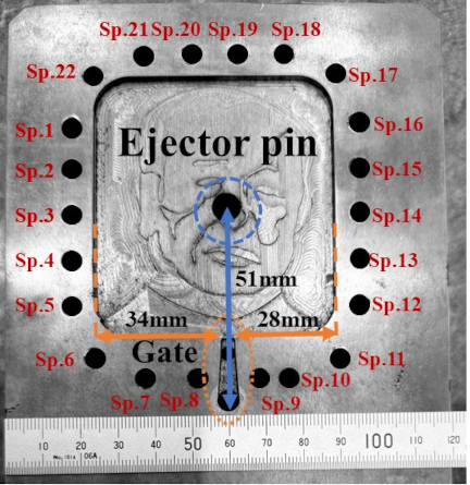
Fig. 1. Schematic representation of the actual mold.
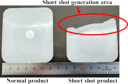
Fig. 2. Normal and short shot products.
2. Experiment
2.1. Experimental Equipment
As shown in Fig. 1, a cavity measuring approximately 60 \(\times\) 80 mm with a thickness of approximately 6 mm was formed in a mold plate with dimensions of 210 \(\times\) 120 mm and a thickness of 45 mm. Around the cavity, 22 spot-facing modifications with a diameter of 5 mm and depth of 0.02 mm were applied. These modifications were confirmed not to affect product quality. Emissivity was standardized by applying a blackbody spray to these locations, allowing for stable and accurate thermal measurements. The 22 measurement points treated with blackbody spray were designated as Sp.1 to Sp.22, as indicated in the figure.
Figure 2 illustrates a comparison between a normally molded product and a defective product exhibiting a short shot. Compared with the normal product, the short-shot specimen has missing portions in the area circled in Fig. 2.
Thermal imaging was performed using an E85 infrared thermal camera (FLIR Systems), which features a resolution of \(384\times 288\) pixels and a measurable temperature range of 253–1,473 K. The camera was mounted on the upper part of the fixed-side mold half at an inclined angle for optimized measurements. Thermal images were captured immediately after the molded product was ejected by the ejector pins, and the captured data were used for subsequent analysis. An overview of the experimental setup is shown in Fig. 3.
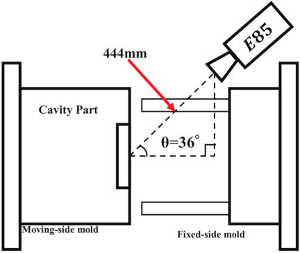
Fig. 3. Experimental schematic.
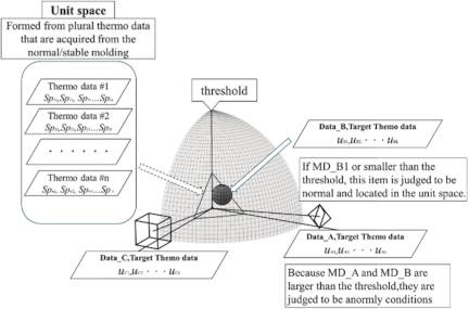
Fig. 4. Concept of MT system.
The injection molding machine used in this study was an SS50 (Sumitomo Heavy Industries, Ltd.), and the mold temperature control unit was an MC5 G1 (Matsui Manufacturing Co., Ltd.). The mold temperature was set to 300 K.
2.2. Anomaly Detection MT Method
Among the various anomaly detection techniques, the MT method is particularly suited for identifying abnormal data from large datasets and offers greater computational efficiency compared to deep learning methods. Therefore, it is used for condition monitoring in manufacturing systems 19,20,21,22. The MT method represents signal data as the Mahalanobis distance (MD) value relative to a reference dataset of normal samples (hereafter referred to as the unit space). The unit space constructed from normal data enables the handling of multidimensional variables. For example, multidimensional parameters, such as acceleration, temperature, and strain, can be reduced to a single scalar MD value, which serves as an index for anomaly detection. In this study, the temperature data from normal molding cycles were used to construct the unit space, and the MT method was applied to determine whether the occurrence of short shots could be detected based on the calculated MD values. A conceptual diagram of the MT system is shown in Fig. 4. The unit space is formed from \(n\) multivariate data acquired under normal/stable forming conditions and serves as the basis for measuring similarity. Under the assumption of three target datasets—Data_A, Data_B, and Data_C—if MD_B is smaller than 1 or the threshold value indicated by the lattice surface, Data_B is considered normal or stable; alternatively, MD_A and MD_C are larger than the threshold, and they are therefore judged as abnormal.
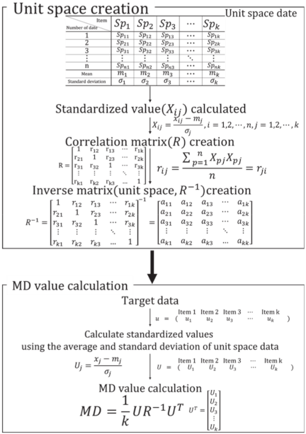
Fig. 5. Calculation process for MD value.
An example of the MD value calculation process is illustrated in Fig. 5.
The MD values were calculated using temperature data obtained from each of the 22 measurement points.
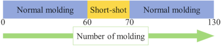
Fig. 6. Experimental procedure.
2.3. Experimental Procedure
To this end, a total of 130 molding cycles were performed as follows: 60 cycles under normal conditions, 10 cycles under short shot conditions, and 60 cycles under normal conditions (Fig. 6). During the defective molding phase, the injection pressure was deliberately reduced (from 100 to 10 MPa) to induce short shots.
Table 1. \(\mathrm{L}_{12}\) orthogonal array.

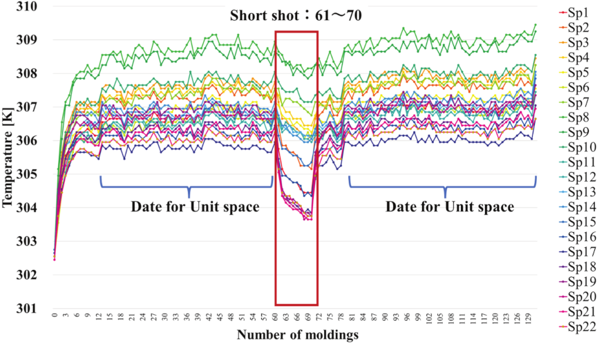
Fig. 7. Temperature variation at all measurement points (130 cycles).
2.4. Item Selection Using Orthogonal Array
The mold insert used in this study included 22 measurement points. Applying the MT method to all the measurement points results in high computational demands and long processing times. Therefore, it is essential to develop a method that reduces the number of measurement points used for MT analysis. To solve this problem, an orthogonal array 23 was used to determine the optimal combination of measurement points aiming to reduce computational load while maintaining detection performance. This approach enables the identification of optimal conditions with a minimal number of experimental trials. In this study, the 22 measurement points were assigned to an orthogonal array, and a sufficient subset of points required for accurate anomaly detection was selected. A two-level L\(_{12}\) orthogonal array (11 factors, 12 experiments) was used in this research. These 22 measurement points were divided into two groups (Sp.1–11 and Sp.12–22) and assigned to the orthogonal array, as shown in Table 1 (Group 1, Nos.1–12; Group 2, Nos.13–24).
In the analysis, “Code 1” in the orthogonal array denotes “use the measurement point,” while “Code 2” denotes “do not use the measurement point.” For example, in trial No.2, Sps.1–5 were used and Sps.6–11 were not. It is important to note that inverse configurations (i.e., use \(\leftrightarrow\) do not use) of measurement point selections do not inherently exist within a single orthogonal array. To address this, a complementary analysis was conducted in which “Code 1” was interpreted as “do not use the measurement point,” and “Code 2” as “use the measurement point,” enabling validation of inverse configurations (trial Nos.1–24). Although larger orthogonal arrays would be required to exhaustively investigate all combinations, reversing usage assignments effectively addresses potential issues such as local optima in parameter selection.
Fig. 8. Short-shot samples.
3. Result and Discussion
3.1. Temperature Measurement Results
Figure 7 presents the thermal transitions at 22 measurement locations over 130 molding cycles. The vertical axis represents the temperature, whereas the horizontal axis indicates the number of moldings. As highlighted in the boxed region during the short-shot events, a marked decrease in temperature was observed at all measurement points. When normal molding resumed, the temperatures returned to baseline levels. Fig. 8 shows the molded specimens from the 63rd and 64th cycles as examples under the short-shot condition applied during cycles 61–70. All short-shot products produced during cycles 61–70 exhibited similar shapes. Consistent with the area circled in Fig. 2, noticeable material deficits are observed along the upper region of the specimens, confirming the occurrence of the same defective shape.
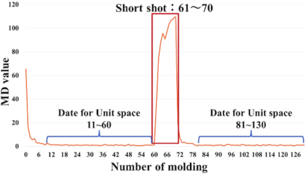
Fig. 9. MD value results.
3.2. MT Method Application Results
For anomaly detection using the MT method, a reference “unit space” must be constructed from normal baseline data. Accordingly, temperature data from cycles 11–60 and 81–130 (totaling 100 cycles) were designated as the normal training data. Fig. 9 presents the results of applying the MT method across all 130 cycles, with the MD value on the vertical axis and the number of moldings on the horizontal axis.
As illustrated in Fig. 9, the MD values increased distinctly during the short-shot period (cycles 61–70), confirming successful defect detection. All short shot cycles were detected, indicating a high level of accuracy. Thus, the detectability and performance of the proposed method are confirmed. A threshold of MD \(=4\) 24 is commonly reported in the literature for anomaly detection, although this may vary depending on experimental conditions.
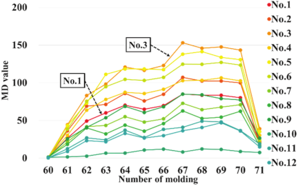
Fig. 10. MD value at occurrence of short shot (Group 1).
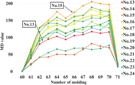
Fig. 11. MD value at occurrence of short shot (Group 2).
3.3. Item Selection Results 1
In Section 2.4, analyses based on orthogonal-array-defined measurement point usage were described: Code 1 \(=\) “use the measurement point,” Code 2 \(=\) “do not use the measurement point.” The 22 measurement points were grouped into Group 1 (Sps.1–11) and Group 2 (Sps.12–22). For example, in Group 1, trial No.1 assigned “Code 1” to all points, meaning Sps.1–11 were all included in the analysis. Figs. 10 and 11 show a comparison of the MD values during the short-shot period for each group.
The highest MD increase in Group 1 occurred in trial No.3 (using Sps.1, 2, 6, 7, and 8), which exceeded that of the full-point analysis (trial No.1). Similarly, in Group 2, trial No.15 (Sps.12, 13, 17, 18, and 19) produced the highest MD, surpassing full-point trial No.13. These results indicate that excluding noisy measurement points improves detection performance. Therefore, Sps.1, 2, 6, 7, 8, 12, 13, 17, 18, and 19 (10 points) reduced the data volume by 55%, while improving MD sensitivity.
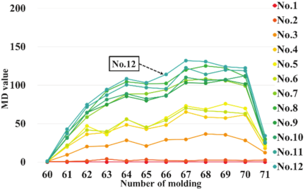
Fig. 12. MD value at occurrence of short shot (Group 1).
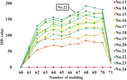
Fig. 13. MD value at occurrence of short shot (Group 2).
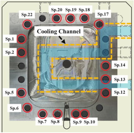
Fig. 14. Item selection results and cooling tube arrangement inside the mold.
3.4. Item Selection Results 2
Section 2.4 also presents an inverse-coding analysis (Code 1 \(=\) “do not use the measurement point,” Code 2 \(=\) “use the measurement point”). Trials 1 and 13 omitted all the measurement points, resulting in a constant MD of 0. Figs. 12 and 13 show a comparison of the MD values during the short-shot period for each group.
Figures 12 and 13 show that trial No.12 (Sps.1, 2, 5, 7, 9, and 10) and No.22 (Sps.12, 13, 14, 19, 20, and 22) produced the highest MD values during the short-shot period, again outperforming full-point trials. These results indicate that excluding noisy measurement points enhances detection performance. Therefore, Sps.1, 2, 5, 7, 9, 10, 12, 13, 14, 19, 20, and 22 (12 points) reduced data volume by 45% while improving MD sensitivity.
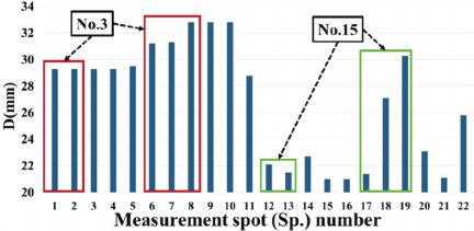
Fig. 15. Result of \(D\) for Section 3.3.
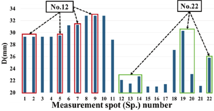
Fig. 16. Result of \(D\) for Section 3.4.
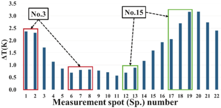
Fig. 17. Result of \(\Delta T\) for Section 3.3.
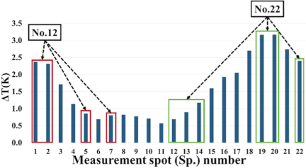
Fig. 18. Result of \(\Delta T\) for Section 3.4.
3.5. Relationship Between Mold Structure and Item Selection Results
Figure 14 shows the locations of the cooling channels inside the mold and 16 measurement points (Sps.1, 2, 5–10, 12–14, 17–20, and 22) selected based on the criteria discussed in Sections 3.3 and 3.4, and 22 measurement points in total. Figs. 15 and 16 illustrate the shortest distances (\(D\)) from the center of each measurement point to the nearest cooling channel.
The justification for this analysis is that, for example, in the event of a temperature fluctuation caused by a short shot, measurement points closer to the cooling channel are likely to return more quickly to the temperature set by the mold temperature controller than points farther away. In other words, the cooling channel is presumed to have a greater influence on nearby points.
Figures 17 and 18 show the relationship between the temperature difference (\(\Delta T\,\)) and the distance \(D\), where \(\Delta T\) is defined as the difference between the average temperature observed during cycles 11–60 and 71–130 (used for standard operation) and the minimum temperature during the 10 short shot cycles (cycles 61–70).
For example, examining Figs. 15 and 17, the relationship between \(D\) and \(\Delta T\) for measurement points Sps.1, 2, and 6–8 in orthogonal experiment trial No.3 reveals that \(\Delta T\) is larger at Sps.6–8, which are farther from the cooling channel, than at Sps.1 and 2, which are closer. As previously noted, it was expected that a smaller \(D\) would result in a quicker return to the set temperature, leading to a smaller \(\Delta T\), however, this trend was not observed. Since a similar tendency was found at other measurement points, the correlation between \(D\) and \(\Delta T\) is considered weak.
In Fig. 17, the combinations of measurement points for trials Nos.3 and 15 share a common feature: they consist of a pairing of one point with a large \(\Delta T\) and another with a small \(\Delta T\). Similarly, in Fig. 18, the combination of trials Nos.12 and 22 also includes points with both high and low \(\Delta T\) values. These combinations, characterized by a contrast in \(\Delta T\) values, yielded high MD values, indicating a strong ability to detect anomalies.
Furthermore, as illustrated in Figs. 17 and 18, the relatively large \(\Delta T\) values observed at Sps.1, 2, 17–20, and 22 are likely due to the geometry of the short shot products. Fig. 19 illustrates the locations of the measurement points selected in Sections 3.3 and 3.4 (Sps.1, 2, 5–10, 12–14, 17, 19, 20, and 22) overlaid on the experimental mold with short-shot products.
As shown in Fig. 19, the upper part of the short-shot product slopes upward toward the upper right of the page. In the mold insert used in this study, the gate position was displaced to the right of the central axis of the cavity. These factors cause an imbalance in the resin flow, resulting in an upward-right inclination of the molded product.
Focusing on Group 1 (Sps.1–11), the areas not reached by the resin were Sp.1 and Sp.2. This likely caused the large temperature differences observed at Sp.1 and Sp.2, and the smaller differences at Sp.4 through Sp.11, as shown in Figs. 17 and 18.
In Group 2 (Sps.12–22), the measurement points not reached by the resin were Sps.17–22. Consequently, the temperature differences at Sps.17–22 were larger than those at the other measurement points, as shown in Figs. 17 and 18.
From these observations, it can be inferred that combining measurement points with both large and small temperature differences improves analysis accuracy while reducing the number of variables. Based on the results of the current experiment and factor selection using an orthogonal array, the essential measurement points for the analysis were determined to be Sps.1, 2, 5–10, 12–14, 17–20, and 22.
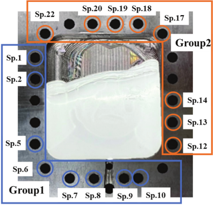
Fig. 19. Mold at short shot occurrence.
Table 2. Selected points for four conditions.

Finally, four conditions are compared in Table 2: (a) the 10-point set from Section 3.3, (b) the 12-point set from Section 3.4, (c) the 16-point union of (a) and (b), and (d) the full 22-point set. Table 2 and Fig. 20 plot the MD values during short-shot events, demonstrating higher MD values for the reduced-point analyses, which indicates improved detection sensitivity.
Figure 21 presents a graph showing the transition of the maximum, minimum, and average MD values under the four conditions when short shots occurred. The horizontal axis represents the number of measurement points used in the analysis.
As shown in Fig. 21, both the maximum and minimum MD values increased as the number of measurement points decreased. A similar trend was observed for the average MD values. These results indicated that a smaller number of strategically selected measurement points can provide a more sensitive response. Therefore, the effectiveness of factor selection using an orthogonal array as a method for efficiently determining measurement locations was validated.
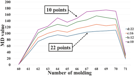
Fig. 20. MD values for four conditions.
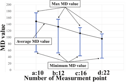
Fig. 21. Transition of MD values for four conditions.
4. Conclusion
In this study, short shots, which are among the primary molding defects in injection molding, were the focus. The feasibility of constructing a condition-monitoring system using the MT method based on noncontact temperature measurements of the mold surface was investigated. To improve the detection performance, an orthogonal array for data selection was applied, and efficient measurement point configurations were evaluated. The major findings are summarized as follows.
-
Application of the MT method successfully enabled detection of short-shot events during molding.
-
Data selection using an orthogonal array reduced the number of measurement points used in the analysis from 22 to 10, decreasing the required data volume and computational load by 55%. This confirms the effectiveness of orthogonal array-based feature selection.
-
The justification for selecting specific measurement points is as follows:
-
Effective detection with the MT method requires a combination of measurement points that show both large and small temperature variations.
-
The magnitude of temperature variation is likely influenced more by the geometry of the short-shot defect than by the mold structure.
-
Based on these results, the potential for developing a practical condition-monitoring system for injection molding processes was demonstrated.
In the future, enabling real-time condition monitoring through data collection and analysis at remote locations will become an important topic. If we conveniently define the limitation of this study, the ideal number of measurement points can be regarded as one. This limitation may be overcome by repeatedly conducting experiments using an orthogonal array. However, because cavity shapes and sizes vary widely in general molds, this study proposes a method for reducing the number of measurement points using an orthogonal array.
- [1] National Institute of Population and Social Security Research, “Population projection for Japan 2021–2070.” https://www.ipss.go.jp/pp-zenkoku/e/zenkoku_e2023/pp2023e_Summary.pdf [Accessed September 11, 2025]
- [2] Cabinet Office of Japan, “Annual report on the ageing society [Summary] FY2024.” https://www8.cao.go.jp/kourei/english/annualreport/2024/pdf/2024.pdf [Accessed September 11, 2025]
- [3] Y. Murata, T. Abe, Y. Sugano, T. Mizusawa, K. Suzuki, K. Ishikawa, and T. Maruyama, “Investigation on relationship between warpage of injection molded products and temperature distribution in a mold,” J. of the Japan Society of Polymer Processing, Vol.20, No.10, pp. 769-775, 2008 (in Japanese). https://doi.org/10.4325/seikeikakou.20.769
- [4] N. Kawada, “Study on condition monitoring technology for digital transformation of manufacturing,” Saitama Institute of Technology Advanced Science Research Laboratory Annual Report, Vol.20, pp. 3-14, 2022 (in Japanese).
- [5] S. Otobe, M. Urano, K. Oizumi, T. Hayashi, A. Ishigami, C. Natthapong, and H. Ito, “Development of ‘expertized AI’ and ‘IoT-based mold’ in mold manufacturing SME,” J. of the Japan Society of Polymer Processing, Vol.31, No.12, pp. 452-455, 2019 (in Japanese). https://doi.org/10.4325/seikeikakou.31.452
- [6] Y. Murata, “Sensor applicated technology to measure molding phenomenon in polymer injection mold,” J. of the Japan Society of Precision Engineering, Vol.81, No.5, pp. 415-420, 2015 (in Japanese). https://doi.org/10.2493/jjspe.81.415
- [7] S. Sakakibara, “Reinforcement of manufacturing industry competitiveness by utilizing robotics, IoT and AI,” J. of the Japan Society of Precision Engineering, Vol.83, No.1, pp. 30-35, 2017 (in Japanese). https://doi.org/10.2493/jjspe.83.30
- [8] Y. Fukushima, T. Suzuki, K. Onda, H. Komatsu, H. Kuroiwa, and T. Kaburagi, “Study on the online monitoring system of barn mark by gas sensor,” Int. J. Automation Technol., Vol.11, No.1, pp. 112-119, 2017. https://doi.org/10.20965/ijat.2017.p0112
- [9] F. Klocke, S. Kratz, T. Auerbach, S. Gierlings, G. Wirtz, and D. Veselovac, “Process monitoring and control of machining operations,” Int. J. Automation Technol., Vol.5, No.3, pp. 403-411, 2011. https://doi.org/10.20965/ijat.2011.p0403
- [10] D. Kurihara, Y. Kakinuma, and S. Katsura, “Sensorless cutting force monitoring using parallel disturbance observer,” Int. J. Automation Technol., Vol.3, No.4, pp. 415-421, 2009. https://doi.org/10.20965/ijat.2009.p0415
- [11] M. Soori, B. Arezoo, and R. Dastres, “Digital twin for smart manufacturing, A review,” Sustainable Manufacturing and Service Economics, Vol.2, Article No.100017, 2023. https://doi.org/10.1016/j.smse.2023.100017
- [12] A. Yokota, “Shashutsuseikei Kisonokiso,” The Nikkan Kogyo Shimbun, 2007 (in Japanese).
- [13] S. Sakano, “A study of bills recognition using MTS,” Quality Engineering, Vol.8, No.3, pp. 58-64, 2000 (in Japanese). https://doi.org/10.18890/qes.8.3_58
- [14] A. M. Yazid, J. K. Rijal, M. S. Awaluddin, and E. Sari, “Pattern recognition on remanufacturing automotive component as support decision making using Mahalanobis-Taguchi System,” Procedia CIRP, Vol.26, pp. 258-263, 2015. https://doi.org/10.1016/j.procir.2014.07.025
- [15] M. Nagao, M. Yamamoto, K. Suzuki, and A. Ohuchi, “A face identification system based on the Mahalanobis–Taguchi System,” Int. Trans. in Operational Research, Vol.8, No.1, pp. 31-45, 2001. https://doi.org/10.1111/1475-3995.00004
- [16] K. Honma, M. Ohkubo, S. Eguchi, and Y. Nagata, “Mahalanobis-Taguchi method for anomaly detection and classification,” Total Quality Science, Vol.8, No.1, pp. 1-13, 2022. https://doi.org/10.17929/tqs.8.1
- [17] J. Shimura, D. Takata, H. Watanabe, I. Shitanda, and M. Itagaki, “Mahalanobis-Taguchi method based anomaly detection for lithium-ion battery,” Electrochimica Acta, Vol.479, Article No.143890, 2024. https://doi.org/10.1016/j.electacta.2024.143890
- [18] Robust Quality Engineering Society, “Quality Engineering Handbook,” The Nikkan Kogyo Shimbun, 2007 (in Japanese).
- [19] Y. Fukushima and N. Kawada, “Online monitoring method for mold deformation using Mahalanobis distance,” Int. J. Automation Technol., Vol.15, No.5, pp. 689-695, 2021. https://doi.org/10.20965/ijat.2021.p0689
- [20] H. Kinjo, Y. Ogawa, Y. Takahashi, N. Kawada, and Y. Fukushima, “Visualization of mold deformation and monitoring system based on Mahalanobis distance,” Quality Engineering, Vol.32, No.2, pp. 32-39, 2024 (in Japanese). https://doi.org/10.18890/qes.32.2_32
- [21] S. Ishida, T. Tahara, W. Iwasaki, and H. Miyamoto, “Evaluation of wire bonding state by thin AE sensor and Mahalanobis-Taguchi System,” Proc. of the Japan Institute of Electronics Packaging Annual Meeting, Vol.30, pp. 187-190, 2016 (in Japanese). https://doi.org/10.11486/ejisso.30.0_187
- [22] Y. Fukushima, Z. Zongyang, A. Sakamoto, and N. Kawada, “Condition monitoring method for injection molding process by waveform analysis,” Proc. of the 22nd Int. Conf. on Advances in Materials & Processing Technologies, 2019.
- [23] K. Hirose and S. Ueda, “Excel de Dekiru Taguchi Mesoddo Kaisekihou nyūmon,” Doyukan, 2003 (in Japanese).
- [24] K. Tamaura, “Yokuwakaru MT System,” Japanese Standards Association, 2009 (in Japanese).
This article is published under a Creative Commons Attribution-NoDerivatives 4.0 Internationa License.