Research Paper:
Automated Determination of Indexing Orientations and Tool Path Generation for 5-Axis Machining of Complex Shapes
Kentaro Matsukawa, Hidenori Nakatsuji, and Isamu Nishida†

Graduate School of Engineering, Kobe University
1-1 Rokkodai-cho, Nada-ku, Kobe, Hyogo 657-8501, Japan
†Corresponding author

In response to the increasing demand for high-mix, low-volume production and the simultaneous shortage of experienced workers, the use of 5-axis controlled machine tools has attracted growing attention. Although complex solid shapes that include free-form surfaces are typically machined using simultaneous 5-axis machining, generation of corresponding numerical control programs continues to depend heavily on the expertise and judgment of experienced operators, rendering parts of the process highly reliant on individual proficiency. In contrast, 5-axis indexing machining involves fewer degrees of freedom compared to simultaneous 5-axis machining. Therefore, by fixing the tool orientation, it achieves easier control and higher machining stability, rendering it suitable for automation. This study developed an automated system that determines both the indexing orientations and tool paths for 5-axis indexing machining, using standard triangulated language format computer-aided design models of complex shapes as input. The system includes a shape removal simulation based on the dexel model, which automatically identifies air-cut regions for each indexing orientation and subsequently generates efficient, waste-free tool paths. Additionally, by leveraging parallel processing on a graphics processing unit, the system accelerates critical operations including tool orientation determination, tool path generation, and air-cut detection, thereby achieving practical computation times for automated process planning.
1. Introduction
In recent years, the manufacturing industry has faced mounting pressure to adapt to rapidly changing customer demands, increasingly diverse market requirements, and shorter product lifecycles. These trends have heightened the need for high-mix, low-volume production and mass customization, which aim to achieve flexibility in production at the same efficiency and cost as traditional mass production 1. Consequently, the development of highly efficient production systems has become a critical issue, particularly for improving productivity in high-mix, low-volume settings. In addition, constraints on human resources, such as the retirement of experienced technicians and a declining younger workforce due to demographic shifts, have intensified, making the automation of manufacturing processes an urgent priority. Within these challenges, automated numerical control (NC) program generation has emerged as a central technological issue in the manufacturing industry. In conventional mass-production systems, the lead time required for process planning is relatively short compared to the overall production time, and most costs are concentrated in machining and setup operations. However, in high-mix, low-volume production, the time required to generate NC programs occupies a larger proportion of the total production time, necessitating automation of this process.
Numerous studies have addressed the automated generation of NC programs, particularly for 3-axis and 5-axis machining. For 3-axis machining, techniques have been proposed to extract geometric features from the target shape, either by recognizing the machining features 2,3,4,5 or by analyzing the removal volume 6,7,8,9. In 5-axis machining, various methods have been proposed for interference avoidance and tool posture optimization using configuration space (C-space) analysis 10,11,12,13,14, as well as tool-path generation methods that consider structural interference 15,16,17,18.
Notably, a previous study 19 proposed a high-precision tool-path generation method for 5-axis machining based on analytical splines and topological structures that enabled the generation of tool paths for arbitrary shapes. This method achieved both shortened machining time and improved accuracy by automatically determining the cutting direction and tool posture through an algorithmic approach.
However, many of these methods rely heavily on specific computer-aided design/computer-aided manufacturing (CAD/CAM) software and assume that machining shapes can be approximated using spline curves. Moreover, users are often required to interactively specify machining regions, select contours, and set entry angles after loading the model. Therefore, the configuration of the tool-path generation parameters depends on manual input and requires expert knowledge to accurately reflect the intended machining strategy. Similarly, in recent years, numerous studies have reported the determination of indexing orientations in 3\(+\)2-axis and 5-axis machining. For example, geometric methods have been proposed to evaluate the machinable range of tool orientations by radially casting rays from a point to construct accessibility cones. Some studies have employed graphics processing unit (GPU) acceleration to perform analyses at high speeds 20. In addition, interactive approaches have been developed to visualize machinable regions on a Gaussian sphere, thereby assisting users in efficiently selecting appropriate tool orientations 21. Although these methods are effective, they remain semiautomated and depend on user judgment and manual operation.
To overcome these limitations, this study proposes an integrated method for the automated determination of indexing orientations and automated NC program generation using standard triangulated language (STL) format CAD models as inputs. In the proposed method, ray casting was performed radially from the centroids of the triangles within the STL model to extract machinable directions that do not interfere with the product shape. Based on the rarity of available cutting directions, an algorithm was constructed to sequentially determine appropriate indexing orientations.
Once the indexing orientations were determined, the tool paths were generated accordingly. A shape-removal simulation using the dexel model was conducted to identify the air-cut regions for each indexing direction. By eliminating the tool paths associated with air cuts, the system automatically corrects the inefficient paths and improves the machining efficiency.
Interference detection between the tool and the dexel model, as well as the update of the dexel state during simulation, was performed using GPU-based parallel computation, significantly reducing the analysis time. Consequently, the proposed method enables the automated generation of NC programs with high practicality and generality, even for the machining of complex shapes involving free-form surfaces.
STL-format CAD models represent surfaces as sets of triangles, each defined by a normal vector and three vertex coordinates 22. Curved surfaces are typically represented using fine triangles, whereas planar surfaces are represented using large triangles. Because of their high compatibility across three-dimensional (3D) CAD systems, STL files are widely used as a standard interchange format. In this method, NC programs can be automatically generated by only inputting an STL-format CAD model into the system, without requiring the user to manually specify machining regions or tool entry angles.
To characterize the interdependencies between the components, the overall workflow of the proposed system is illustrated in Fig. 1. The system uses an STL-format CAD model as the input, performs orientation analysis to determine indexing orientations, generates tool paths, and applies a dexel-based shape simulation for air-cut detection and correction. By integrating these processes, NC programs for 5-axis indexing machining were generated automatically.
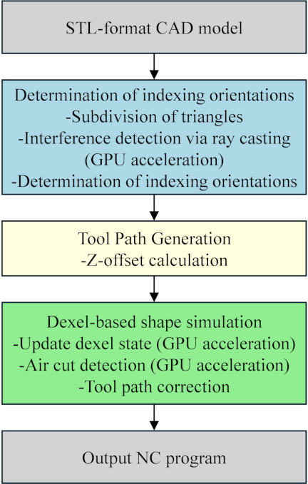
Fig. 1. Workflow of the proposed system.
The remainder of this paper is organized as follows. Section 2 provides an overview and details of the proposed algorithm for determining indexing orientations. Section 3 explains the air-cut detection and tool-path correction using a dexel-based shape simulation. Section 4 presents machining experiments and results to demonstrate the effectiveness of the proposed approach.
2. Automated Determination of Indexing Orientations for 5-Axis Machining
2.1. Overview of the Algorithm
This section describes the challenges associated with conventional methods for machining complex shapes, including freeform surfaces, and outlines the novelty and structure of the proposed algorithm for automated determination of indexing orientations.
Complex shapes, including freeform surfaces, are typically machined using simultaneous 5-axis machining. This method allows all axes to be controlled simultaneously, offering high degrees of freedom and flexible adaptation to complex shapes. However, the generation of NC programs for simultaneous 5-axis machining requires continuous control of the tool orientation and prevention of collisions, which in turn demands advanced expertise and technology, posing a significant barrier to full automation.
To address these challenges, this study focuses on 5-axis indexing machining, which is inherently more compatible with automation owing to its reduced control complexity. In 5-axis indexing machining, the tool orientation remains fixed during each operation, and 3-axis machining is performed by incrementally adjusting the indexing angles. This technique simplifies tool posture control compared to simultaneous 5-axis machining and facilitates collision prevention with tool holders, vises, and other components, as well as tool-path generation. However, selecting suitable indexing orientations in this context relies heavily on the experience of skilled operators. For complex shapes that include free-form surfaces, comprehensively and efficiently extracting all feasible machining directions is challenging. Although several studies have addressed the automated determination of indexing orientations, their applicability has been confined to simple geometries, rendering them ineffective for complex shapes involving freeform surfaces 23,24.
The novelty of this study lies in its ability to efficiently and comprehensively extract viable indexing orientations through GPU-parallelized ray casting-based interference detection performed on STL-format CAD models. Furthermore, the proposed algorithm is applicable not only to simple shapes but also to complex geometries that include overhangs and free-form surfaces, enabling automated process planning for a wide range of product shapes.
This study proposes an algorithm to efficiently determine the indexing orientations required for 5-axis indexing machining. This method sequentially selects tool orientations based on the rarity of feasible directions within a specified angular resolution, thereby suppressing redundant orientations. In this sense, the algorithm practically extracts the minimal necessary orientations rather than guaranteeing a mathematically optimal minimum. This approach is motivated by two key considerations:
-
I.
Reduction of computational cost
To calculate the tool paths, separate tool paths must be computed for each indexing direction. Excessive indexing increases the computational load and prolongs processing time.
-
II.
Reduction of machining error
A greater number of indexing operations implies more frequent changes in the machine posture, which may introduce cumulative positioning errors owing to machine-specific characteristics and control precision, potentially degrading the machining quality.
The proposed method performs radial ray casting from the centroid of each triangle in an STL-format CAD model to detect interference. This technique allows for the efficient exploration of feasible machining directions and determination of appropriate indexing orientations. Consequently, all machining regions can be processed with a minimal number of indexing operations, enabling the efficient 5-axis indexing machining of complex shapes.
Even in the roughing stage, the system determines the indexing orientations based on triangles representing the final product surface with a machining allowance. This strategy ensures that all the surface elements of the product can be accessed without interference, thereby preventing uncut regions. By adopting the product geometry as a reference in both roughing and finishing processes, the system yields consistent accessibility evaluation and reliable process planning. This approach differs from conventional methods, which often determine tool orientations with respect to the stock geometry.
The automated determination of indexing orientations in the proposed method follows the procedure described in the subsequent subsections.
Input: STL-format CAD model
Step 1: Subdivision of triangles and centroid offset processing
In this study, interference detection for machining directions is performed by ray casting from the centroid of each triangle. Therefore, the density of the sampling points significantly affects the accuracy of direction evaluation. However, when an STL-format CAD model contains large triangles, the overall shape may not be sufficiently sampled, potentially reducing the precision of indexing direction detection for the local geometry. To address this limitation, the system subdivides any triangle whose size exceeds the feed pitch during roughing. Furthermore, for each triangle, the system computes its centroid and slightly offsets it in the direction of its surface normal. These offset points, referred to as sampling points, are shifted to avoid lying directly on the surface of the original triangle, thereby preventing false detections during subsequent interference analysis.
Step 2: Interference detection via ray casting
Subsequently, for each offset centroid (sampling point) obtained in Step 1, the rays are radially cast in various directions at the specified angular intervals. For each ray, the system performs interference detection against all triangles in the CAD model, extracting only the directions with no interference. This process allows the identification of feasible interference-free directions associated with each sampling point. Because the interference check for each point is independent, this process is efficiently parallelized using GPU computations to achieve high-speed performance.
Step 3: Determination of indexing orientations
Based on the results of Step 2, each sampling point is associated with one or more interference-free directions. In Step 3, appropriate indexing orientations are selected sequentially from among the candidates. For each feasible direction, the set of unprocessed sampling points that could be approached from that direction is collected. The importance of each point is evaluated based on the rarity of its accessible directions, and points that can be machined from fewer directions are considered more important. A score is then computed for each candidate direction by summing the importance weights of the reachable unprocessed points. The direction with the highest score is selected as the next indexing orientation. This process is repeated until all points are marked as processed or all candidate directions have been exhausted. Thus, the algorithm automatically determines efficient indexing orientations while considering the rarity of the machining directions.
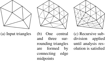
Fig. 2. Subdivision of triangles.
2.2. Details of the Algorithm
2.2.1. Subdivision of Triangles and Centroid Offset Processing
In the proposed algorithm for the automated determination of indexing orientations, the first step involves preprocessing the STL-format CAD model by subdividing the triangles and applying an offset to their centroids. This step is crucial to ensure the accuracy and robustness of the subsequent interference detection process.
For each triangle, the lengths of the three edges are first computed. If the longest edge exceeds the feed pitch during roughing, the triangle is subdivided. Subdivision is performed by computing the midpoints of each edge and connecting these points to form four smaller triangles from the original triangle. The feed pitch is one of the primary factors that determine the upper bound of machining accuracy. By setting the subdivision threshold based on the feed pitch, the geometric errors introduced by discretization are kept within machining tolerances. Although a finer analysis resolution improves the geometric approximation accuracy, it also increases the number of triangles, leading to a higher computation time and memory usage. Conversely, a coarser resolution improves the computational efficiency but may reduce the approximation accuracy, potentially affecting the reliability of the indexing orientation determination.
Figure 2(a) shows the input triangles. As illustrated in Fig. 2(b), three new points are created at the midpoints of the edges, and connecting these points forms a central triangle and three surrounding triangles. Thus, the original triangle is divided into four smaller triangles. This subdivision process is applied recursively until the length of the longest edge in each triangle is less than or equal to the feed pitch during roughing (Fig. 2(c)).
After subdivision, the centroid of each triangle is computed, and a small offset is applied. This offset is essential for avoiding false positives caused by self-intersection during interference detection, where the ray may be incorrectly judged to intersect the triangle from which it originates. To prevent this discrepancy, the surface normal vector \(\boldsymbol{n}\) of the triangle is computed, and the centroid position vector \(\boldsymbol{v}\) is offset in the direction of the normal as follows:
Here, \(\varepsilon\) is a small positive constant, typically on the order of \(10^{-4}\) mm. Because the offset centroid \(\boldsymbol{v}'\) no longer lies on the surface of the original triangle, self-intersection errors during ray casting can be effectively prevented. Additionally, because the offset is extremely small, its effect on the overall geometry is negligible. Fig. 3 illustrates this concept. Without an offset, a ray from the centroid is immediately judged to intersect the originating triangle (self-interference). By shifting the centroid slightly along the normal vector by \(\varepsilon\cdot\boldsymbol{n}\), such false detections can be effectively prevented.
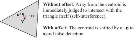
Fig. 3. Self-intersection.
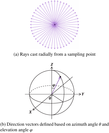
Fig. 4. Definition of direction vectors and schematic illustration of ray casting.
2.2.2. Interference Detection via Ray Casting
As a preprocessing step, the feasible machining directions are explored by radially casting rays from each sampling point. As illustrated in Fig. 4(a), the central point represents a sampling point from which many rays are emitted into the 3D space while varying the direction at fixed angular intervals (Fig. 4(b), shown in purple). This operation enabled interference evaluation in all directions surrounding the sampling point.
However, the range of candidate directions is constrained by the rotational axis limits of the machine tool. Therefore, in this study, only directions within a predefined angular range are considered, based on the practical limitations of actual machining systems.
Each ray direction vector \(\boldsymbol{d}\) is defined by an azimuth angle \(\theta\) and an elevation angle \(\varphi\), as follows:
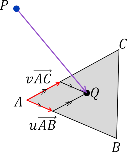
Fig. 5. Interference detection via ray casting.
Here, the azimuth angle \(\theta\) represents the rotation angle in the \(XY\)-plane, and the elevation angle \(\varphi\) indicates the inclination from the \(Z\)-axis (Fig. 4(b)). Using these direction vectors, ray casting is performed to extract the directions that do not intersect with the product geometry.
Subsequently, for each ray, interference detection is performed against all triangles that constitute the CAD model. This process is based on the constraint that the tool cannot approach from a direction intersecting the product. The goal is to identify the indexing orientations from which the tool can access the surface without collision.
Interference detection is conducted by computing the intersections between each ray and the triangles of the CAD model. As shown in Fig. 5, the algorithm determines whether a ray originating from point P intersects the interior of an arbitrary triangle ABC. If an intersection is detected, the corresponding direction is considered obstructed and excluded from the list of valid approach directions.
As illustrated in Fig. 5, triangle ABC lies on the plane spanned by vectors \(\overrightarrow{AB}\) and \(\overrightarrow{AC}\), with vertex A as the reference point. If the intersection point Q of a ray and the triangle lies within the triangle, its position can be expressed as
For point Q to lie inside the triangle, the following conditions must be satisfied:
A ray is represented by a starting point P and direction vector \(\boldsymbol{d}\), and is defined as
For the ray to intersect the triangle, values of \(t\ge 0\) and \(u\), \(v\) must exist such that both Eqs. \(\eqref{eq:3}\) and \(\eqref{eq:5}\) describe the same point Q. Furthermore, the intersection point is valid only if the conditions in Eq. \(\eqref{eq:4}\) are satisfied. In this case, the ray is considered to interfere with the triangle.
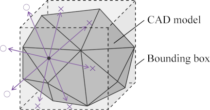
Fig. 6. Schematic illustration of feasibility check considering tool overhang length.
Using this formulation, interference checks are performed against all triangles in the CAD model. If an intersection is detected with even one triangle, the corresponding ray direction is classified as an interference. Conversely, if no intersections are found with any triangle, the ray direction is considered non-interfering, and thus represents a candidate direction from which the tool can approach the part.
In addition, to account for the user-specified tool overhang length, each candidate direction is further validated. The tool overhang length directly affects the number of feasible orientations: a shorter overhang length limits tool accessibility and reduces the number of feasible orientations, whereas a longer overhang length allows more orientations. If a point located at a specified distance along the ray from the sampling point lies outside the bounding box of the product model, that direction is considered infeasible and is excluded. This step ensures that even if a direction is geometrically interference-free, it is rejected if the tool cannot physically reach the target surface, allowing the system to select only machining directions that are feasible in practice.
Figure 6 illustrates the concept of feasibility evaluation based on the tool overhang length. A ray (purple line) is cast from a sampling point, and the approach direction is judged to be feasible or infeasible, depending on whether the point located at a specified distance along the ray remains inside the bounding box of the product model.
For complex shapes containing many freeform surfaces, which are the primary targets of this study, the number of triangles in the CAD model becomes extremely large. Consequently, the interference detection process can be computationally expensive. To address this challenge, this study proposes the use of parallel processing on a GPU to significantly reduce analysis time.
Although GPUs were originally developed for graphics processing, they have been increasingly applied to scientific computations owing to their ability to execute numerous identical computations in parallel. When utilizing a GPU, data must be transferred from the host memory (central processing unit; CPU) to the device memory (GPU) before execution, and the results must be transferred back afterward. Although this memory transfer introduces an overhead, the overall processing efficiency improves significantly when many computations are performed in parallel or when the computational load per task is high.
In this study, the vertex coordinates of all the triangles in the CAD model, coordinates of the sampling points, and direction vectors of the rays are transferred in advance to the GPU memory. Each GPU thread independently performs interference detection (i.e., intersection tests between rays and triangles) to compute the feasible \(Z\)-axis positions of the tool at each \(XY\) location.
Specifically, each thread evaluates all the ray directions cast radially from a given sampling point and performs intersection tests with triangles. By executing this interference detection process for all ray directions in parallel across threads, high-throughput parallel computation is achieved. The results from all threads are then transferred back to the CPU, enabling high-speed interference analysis. Through this GPU-accelerated approach, the proposed method achieves a substantial reduction in the analysis time compared with conventional CPU-based sequential processing.
2.2.3. Determination of Indexing Orientations
Based on the results of the interference detection in Step 2, interference-free indexing directions (i.e., ray directions) have been obtained for each sampling point. In this step, these results are used to sequentially determine a set of indexing orientations that efficiently and comprehensively cover unprocessed points while considering the rarity of feasible machining directions.
First, for each feasible machining direction, \(S_i\), the system extracts a set of sampling points, \(P_i\), that can be approached from that direction. Subsequently, for each point \(p\in P_i\), the system computes in advance the total number of feasible directions \(\vert D_p\vert\) from which it can be accessed. This study defines the weight of point \(p\) as the reciprocal of this number:
This weighting ensures that points that can only be accessed from a limited number of directions are given a higher priority. For each direction \(S_i\), the system computes a score by adding the weights of the unprocessed points in \(P_i\), as defined by the following equation:
The direction \(S_i\) that yields the maximum score is selected as the next indexing orientation. The corresponding point set is marked as processed.
This process is repeated iteratively until all sampling points have been marked as processed or all candidate directions have been exhausted. Through this repetition, the algorithm automatically generates a set of efficient indexing orientations, prioritized rare machining directions, and enabled highly efficient 5-axis indexing machining.
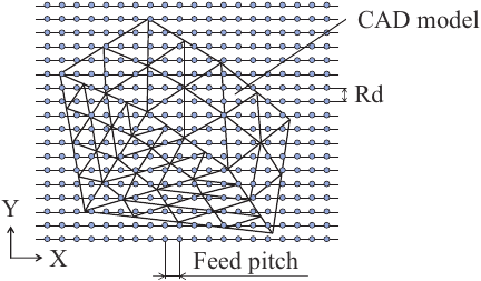
Fig. 7. Tool position on the \(XY\)-plane in scanning machining.
3. Air-Cut Detection and Automated Tool-Path Correction Using Dexel-Based Shape Simulation
3.1. Automated Tool Path Generation
In the case of complex shapes that include freeform surfaces, extracting machining features from CAD models and designing machining processes based on conventional contour machining strategies are often challenging 2,3,4,5,6,7,8,9. Therefore, this study employs scanning line machining using an STL-format CAD model of the product.
In scanning line machining, tool paths can be generated by determining only the \(Z\)-axis offset based on the interference between the product geometry and tool, given fixed tool positions in the \(XY\)-plane 25. Accordingly, the system first determines the tool positions in the \(XY\)-plane based on the tool radius step-over distance Rd and feed direction resolution (pitch), as illustrated in Fig. 7.
Subsequently, the system calculates the \(Z\)-axis offset for each \(XY\) tool position. In this study, a geometric analysis is conducted for a ball end mill. For such tools, the \(Z\)-offset is defined as the height at which the spherical tool tip contacts a triangle of the product surface. Specifically, the system geometrically computes the \(Z\)-coordinate corresponding to the highest valid contact between the spherical surface of the tool and a triangle, considering the following three types of contact:
-
Contact between the sphere and a triangle face (Fig. 8(a));
-
Contact between the sphere and a triangle edge (Fig. 8(b));
-
Contact between the sphere and a triangle vertex (Fig. 8(c)).
The geometric relationship for the face contact is shown in Fig. 9. In 3D space, given a unit normal vector \(\vec{n}\) and point A on the plane, the projection of point P onto the plane is denoted by H. The following relationship holds:
Because the radius of the sphere is equal to the tool radius \(r\), the distance from the center point P to the contact point H must satisfy
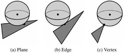
Fig. 8. Positional relationship between tool and triangle contacts.
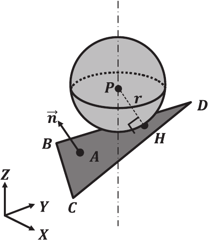
Fig. 9. Geometric relationship between sphere and plane.
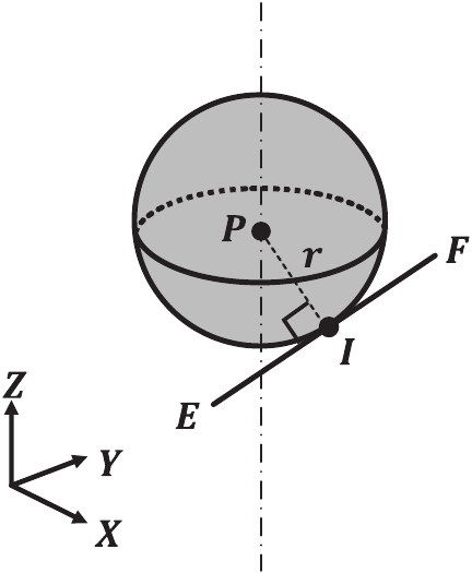
Fig. 10. Geometric positional relationship between spheres and edges.
Furthermore, the contact point must lie inside the target triangle, which requires that
The edge-contact relationship is shown in Fig. 10. Let I be the foot of the perpendicular dropped from point P to edge segment EF. The orthogonality condition is as follows:
Similarly, the radius condition is
To ensure that the contact lies within the edge segment, the following must hold:
Note that contact with vertices is considered a special case of edge contact.
The system evaluates all the triangles and their edges for each tool position determined in the \(XY\)-plane. By identifying the point P that satisfies Eqs. \(\eqref{eq:8}\)–\(\eqref{eq:13}\) and has the maximum \(Z\) value, the system determines the appropriate \(Z\)-axis tool height.
Although the tool paths are generated at equal intervals on the \(XY\)-plane, a simple uniform distribution may cause overcutting on steep or inclined surfaces. To address this issue, the proposed system further subdivides the intervals between adjacent tool positions and performs detailed tool–workpiece contact calculations at each subdivided point. The \(Z\)-height of the tool tip is then determined from these evaluations, which prevents overcutting and ensures the accurate machining of complex regions. In addition, redundant tool contact points produced during this process are automatically identified and eliminated through a dexel-based shape simulation, which detects air cuts and removes unnecessary paths, thereby improving efficiency.
Moreover, the machining accuracy of the proposed method is inherently bounded by the feed pitch and resolution of the input CAD model. Consequently, the geometric error introduced by discretization never exceeds the feed pitch, ensuring sufficient precision for practical machining.
3.2. Shape Simulation Using the Dexel Model
In 5-axis indexing machining, the tool paths are generated sequentially for each indexing orientation. However, this often results in the generation of redundant tool paths for regions that have already been removed in previous operations. This leads to air cutting, in which no material is removed, thereby increasing machining time and reducing the overall efficiency.
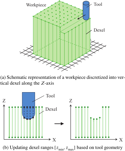
Fig. 11. Conceptual illustration of the dexel model and tool interference.
To address this issue, the system implements a machining simulation using the dexel model, which continuously records and updates the material removal state based on tool entry. This method allows the system to automatically identify the air-cut regions and correct the tool paths accordingly. As shown in Fig. 11(a), the dexel model represents the workpiece geometry as a set of parallel line segments aligned in the \(Z\)-direction. When the tool penetrates the model, the dexel line segments within the affected region are updated based on the interference detection, as illustrated in Fig. 11(b). Each dexel line is characterized by its current minimum and maximum \(Z\)-values \([{z}_{\min},{z}_{\max}]\), which are updated dynamically to reflect material removal. Compared with voxel-based models, the dexel model enables a smoother and more precise simulation of geometric changes.
For each computed tool position, the system evaluates whether the corresponding dexel segment is geometrically contained in the tool shape. If not contained, the position is skipped, thereby eliminating unnecessary air cuts and producing a more efficient tool path.
The dexel model is a well-established geometric representation technique that is widely used to understand material removal in machining simulations 26,27,28. However, this study uniquely applies the dexel model to track tool interference and identify air-cut regions in the context of 5-axis indexing machining. The system dynamically eliminates unnecessary tool-path segments from the NC program by utilizing this interference history.
In this study, the dexel-based machining simulation is not executed simultaneously with tool-path generation. Instead, the dexel-based simulation is applied sequentially to the tool paths generated for each indexing orientation after all the orientations have been determined, thereby detecting and removing air cuts.
The novelty of this approach is that the system updates the machining history of the dexel model for each tool position generated at a specified indexing orientation. This enables automated skipping of noncontributory tool paths during the tool-path generation process.
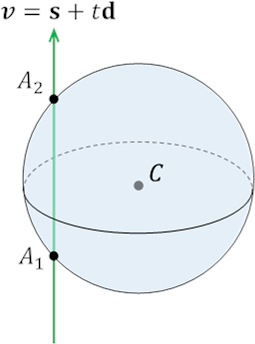
Fig. 12. Interference between a sphere and a dexel.
The following section describes in detail how intersections are computed between each dexel line segment and the tool, assuming that the tool is either spherical or cylindrical in shape.
3.2.1. Geometric Processing Between a Spherical Tool and a Dexel
This study considered a cutting tool with a spherical tip, such as a ball end mill. To determine whether this type of tool interferes with the workpiece (represented by a dexel), the intersection between the sphere and dexel must be computed. As shown in Fig. 12, this study analyzes the case in which the dexel penetrates the spherical tool shape. In this scenario, the system analytically calculates the intersection points between the dexel, which extends toward the sphere from each \(X\)–\(Y\) coordinate, and the sphere surface. The following section describes the method for deriving the intersection points between the sphere and dexel.
In a 3D space, consider a sphere with radius \(r\) and center positions \(\boldsymbol{C}=(x_C,y_C,z_C)\), and a dexel defined as a ray with a starting point \(\boldsymbol{s}=(x_s, y_s, 0)\) and direction vector \(\boldsymbol{d}=(0,0,d_z)\). The dexel can be represented as
The conditions for the sphere and dexel to intersect are given as follows:
That is,
By rearranging Eq. \(\eqref{eq:15}\) with respect to \(t\), this study obtains the following quadratic equation:
An intersection exists if and only if the discriminant of this quadratic equation is non-negative. Therefore, the geometric condition for interference is
From Eq. \(\eqref{eq:16}\), the parameter \(t\) corresponding to the intersection point can be obtained as
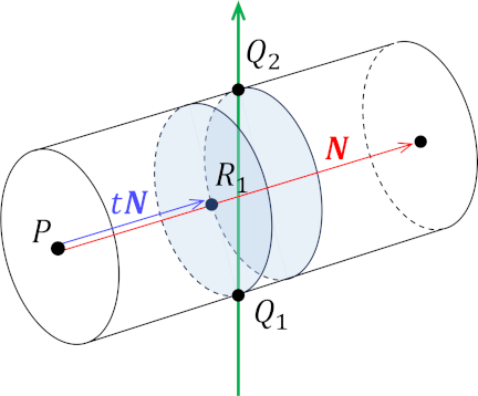
Fig. 13. Interference between a cylinder and a dexel.
Thus, the \(Z\)-coordinate of the intersection point is
3.2.2. Geometric Processing Between a Cylindrical Tool and a Dexel
As illustrated in Fig. 13, this section considers interference detection between a cylindrical tool and a dexel. For simplicity, tool position \(P\) is shifted to the origin of the coordinate system. Let \(Q_1(x_0,y_0,z_1)\) and \(Q_2(x_0,y_0,z_2)\) be the entry and exit points at which the dexel intersects the cylindrical tool. Each of these points lies on a cross-sectional circle of the cylinder.
Let \(R_1\) and \(R_2\) be the centers of the corresponding circular cross-sections. The length from each center point \(R\) to its respective contact point \(Q\) corresponds to the radius \(r\) of the cylindrical tool:
Let the normal vector of the cylinder axis be \(\vec{N}=(N_x,N_y,N_z)\). Because each circular cross-section is orthogonal to the cylinder axis, the following condition holds:
Because the center \(R\) lies along the cylinder axis, it can be expressed using a scalar parameter \(t\) (\(0\le t\le 1\)) as follows:
Substituting this into Eq. \(\eqref{eq:21}\) and simplifying yields the following expression:
Let \(\left\Vert\vec{N}\right\Vert^2=N_x^2+N_y^2+N_z^2\), then solving for \(t\) gives
Substituting Eq. \(\eqref{eq:22}\) into Eq. \(\eqref{eq:20}\) and simplifying yields
Rearranging this relationship with respect to z, this study obtains the following quadratic equation:
Thus, the \(Z\)-coordinates of the intersection points \(Q\) are given by
Finally, if the actual tool position is \(P=(x_p,y_p,z_p)\), the \(Z\)-coordinates of the intersection points are shifted accordingly:
3.3. Dexel Data Structure and Parallel Updates Using GPU Processing
The dexel model is a data structure that stores a set of occupied intervals, \([{z}_{\min},{z}_{\max}]\) along the \(Z\)-axis for each \(XY\)-coordinate defined at a given resolution. This structure enables fast and memory-efficient geometric processing, including interference detection and shape simulation.
To ensure efficient memory access during parallel execution on a GPU, the dexel model was implemented as a one-dimensional array. The \(XY\)-plane is discretized into a grid consisting of \({N}_{x}\) cells in the \(X\)-direction and \({N}_{y}\) cells in the \(Y\)-direction. Each 2D cell index \((x,y)\) is converted into a linear index using the following formula:
This index uniquely determines the starting memory address for storing the \(Z\)-direction data for each cell. Each cell can store up to \(N\) segments representing the occupied intervals along the \(Z\)-axis. A single segment is defined by a floating point pair \(({z}_{\min}^{(n)},{z}_{\max}^{(n)})\), which indicates its start and end points.
The segmented data for each cell are stored in a contiguous block of memory. If \(i\) is the linear index of the cell and \(n\) is the index of a segment within that cell, the segment is stored in memory positions:
A fixed-length region of size \(2N\) is preallocated to every cell. As the number of segments varies by location, the actual number of segments stored per cell depends on the geometry of the model.
In the GPU implementation, each GPU thread is assigned to a single grid cell in the \(XY\)-plane. It evaluates the interference between the tool and the dexel(s) in that cell. When interference is detected, the affected \(Z\)-interval is immediately updated in memory to reflect the resulting shape change.
This update process, which adjusts the occupied regions along the \(Z\)-axis, is essential for accurately tracking the evolution of the machined shape. By assigning one thread per cell and updating the dexel model in parallel across the spatial regions, the system achieves high-speed and efficient dynamic shape simulation.
Each thread executes the following steps:
-
Retrieve the dexel data assigned to its cell.
-
For every tool position along the tool path, perform the following:
-
(a)
Retrieve the tool’s current position and shape parameters.
-
(b)
Evaluate whether the tool intersects with the assigned dexel.
-
(c)
If interference is detected, update the occupied interval \([{z}_{\min},{z}_{\max}]\) accordingly.
-
(a)
Using this approach, each dexel cell in the \(XY\)-plane is handled using a dedicated GPU thread, enabling spatial parallelization. Simultaneously, each thread sequentially processes all the tool positions for its assigned dexel, dynamically reflecting the changes in the machined geometry. As a result, the system efficiently updates the dexel model for complex cutting operations by leveraging GPU parallelism.
When interference is detected between the tool and dexel, the manner in which the \(Z\)-direction segments are updated depends on the position and extent of the interference. These interference conditions can be broadly classified into four representative patterns, each of which requires a different update strategy.
These patterns and their corresponding updating methods are explained in detail in the following sections. The blue and black segments in Fig. 14 represent the tool geometry and dexel intervals, respectively.
3.3.1. Partial Interference at the Upper End of the Dexel
Figure 14(a) illustrates a case in which the tool partially interferes with the upper end (\({z}_{\max}\)) of the dexel segment. In this case, the upper portion of the segment is removed. The system reflects the material removal by decreasing the value of \({z}_{\max}\) to the contact position of the tool. The lower end \({z}_{\min}\) remains unchanged, and the lower part of the segment is retained as a valid uncut region.
3.3.2. Partial Interference at the Lower End of the Dexel
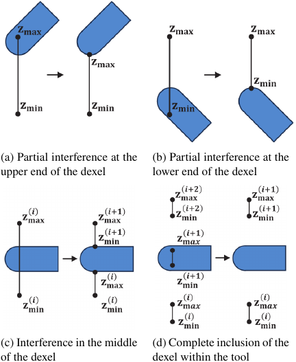
Fig. 14. Classification of interference cases between the tool and the dexel.
Figure 14(b) shows the case in which the tool partially interferes with the lower end (\({z}_{\min}\)) of the dexel segment. In this case, the lower portion of the segment is removed, and the system updates \({z}_{\min}\) by increasing it to the contact position of the tool. The upper end \({z}_{\max}\) is preserved, allowing the upper part of the segment to remain in a valid uncut region.
3.3.3. Interference in the Middle of the Dexel
This occurs when the tool interferes with the middle of the dexel segment. This interference removes a portion of the segment, leaving both the upper and lower regions uncut. To preserve the uncut regions accurately, the system splits the original segment into two segments.
As shown in Fig. 14(c), if the original segment \(i\) spans the ranges \([{z}_{\min}^{(i)},{z}_{\max}^{(i)}]\), and the tool interference ranges \([{z}_{\mathrm{tool\_min}},{z}_{\mathrm{tool\_max}}]\) lie within this interval, two new segments are defined.
-
Upper remaining segment:
\begin{equation} \label{eq:31} {z}_{\min}^{(i+1)}={z}_{\mathrm{tool}_{\max}},\quad{z}_{\max}^{(i+1)}={z}_{\max}^{(i)}. \end{equation} -
Lower remaining segment:
\begin{equation} \label{eq:32} {z}_{\min}^{(i)}={z}_{\min}^{(i)},\quad{z}_{\max}^{(i)}={z}_{\mathrm{tool}_{\min}}. \end{equation}
This ensures that the middle portion removed by the tool is excluded, whereas the uncut upper and lower regions are precisely retained in the dexel model. The system dynamically applies this segmentation, allowing it to accommodate complex variations in the cutting geometry.
3.3.4. Complete Inclusion of the Dexel Within the Tool
Figure 14(d) represents the case in which the tool’s interference range fully encompasses the dexel segment, making it entirely removable. When the dexel segment \([{z}_{\min}^{(i)},{z}_{\max}^{(i)}]\) is fully contained within the occupied regions \([{z}_{\mathrm{tool\_min}},{z}_{\mathrm{tool\_max}}]\), the system removes the segment from the data structure.
This prevents the unnecessary computation of segments that have already been removed. In implementation, memory compaction is performed by shifting valid segments forward to overwrite deleted entries, thereby eliminating unnecessary data and improving processing efficiency.
3.4. Shape Information Retention in Multi-Process Machining Using Multiple Tools with the Dexel Model
The proposed system enables consistent management of shape information across multiple machining processes, such as roughing with a square end mill, followed by finishing with a ball end mill, by leveraging the dexel model.
The \(Z\)-direction segment data, representing the regions removed during the roughing process, are preserved directly within the dexel array. In subsequent processes, this dexel state is reused as the initial condition, enabling accurate air-cut detection and effective removal or shortening of unnecessary tool paths based on the machining history.
For example, consider a case in which most of the material is removed by roughing with a square end mill, and then a ball end mill is used to finish the curved surfaces. Because the volume removed from the roughing process is retained in the dexel model, the system can restrict interference detection during ball end milling to only the remaining uncut regions, thereby generating tool paths that effectively eliminate air cuts.
In conventional CAM systems, it is necessary to reconstruct the workpiece geometry for each machining process. In contrast, the proposed method inherently retains the updated geometry between operations, allowing seamless transition of shape information across processes. This eliminates the need for redundant shape regeneration and supports a practical automated process planning framework for multi-process machining.
This architecture is particularly beneficial for high-precision multi-process machining of freeform surfaces and for efficient machining strategies using multiple tools, as it contributes to maintaining consistency in shape information and reducing dependence on operator expertise.
3.5. Air Cut Detection and Automated Tool Path Correction Using the Dexel Model
This section describes the method for automatically detecting air cuts along the tool path and correcting the path accordingly. In the proposed system, as illustrated in Fig. 15(a), the tool position is considered a valid machining point if the tool interferes with at least one dexel within its range.
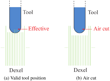
Fig. 15. Air cut detection.
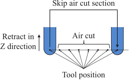
Fig. 16. Tool retraction during air cut segments.
Conversely, as shown in Fig. 15(b), if the tool does not interfere with any dexel, then the position is identified as an air cut, and the tool position is regarded as unnecessary.
Interference detection in this context is performed based on the geometric intersection between the tool shape and the dexel, as described in Section 3.2.
The air-cut detection process is accelerated using GPU-based parallel processing, in which the interference with all dexels is evaluated simultaneously for each tool position. Each GPU thread is assigned a specific tool position, and the intersections with all dexels were evaluated to determine whether the position results in an air cut.
As shown in Fig. 16, the system evaluates the presence or absence of air cuts at each tool position. If the length of a continuous air-cut segment exceeds a predefined threshold, the tool is temporarily retracted in the \(Z\)-direction, and the system skips the corresponding segment.
This approach enables the automated generation of NC programs that effectively reduce unnecessary tool movements and eliminate segments that do not contribute to the actual machining.
The reason for introducing a threshold is that inserting retraction motions for every short air-cut segment may result in intermittent and redundant tool paths, potentially reducing the machining efficiency. In such cases, allowing the tool to pass through short air-cut segments without retraction is often beneficial because it reduces the overall machining time.
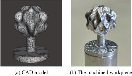
Fig. 17. Product model and machined result in Case 1.
4. Case Study
Two case studies were conducted to evaluate the effectiveness and versatility of the proposed system.
-
I.
Case 1
The first case study targeted an STL-format CAD model, as shown in Fig. 17(a) (diameter: 20.0 mm, height: 27.4 mm). An NC program was automatically generated using the proposed system and used for machining. The workpiece material was aluminum alloy A2017, and machining was performed using a Pocket NC V2-10 manufactured by NK Works Co., Ltd. The system generates the roughing tool path shown in Fig. 18, based on the machining conditions listed in Table 1. The corresponding machining results are shown in Fig. 17(b).
-
II.
Case 2
To assess the applicability of the proposed method to more complex geometries, an additional experiment was conducted using the freeform surface model shown in Fig. 19(a) (diameter: 20.0 mm, height: 22.4 mm). The same machining center and workpiece material were used, and the roughing tool path was generated under the same machining conditions listed in Table 1. A portion of the generated tool path is illustrated in Fig. 20, and the machining results are shown in Fig. 19(b).
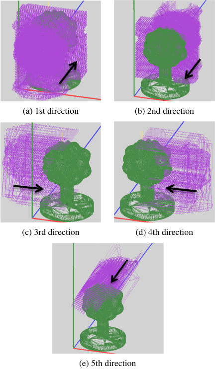
Fig. 18. Roughing tool path with ball end mill in Case 1.
Table 1. Machining conditions for case study.

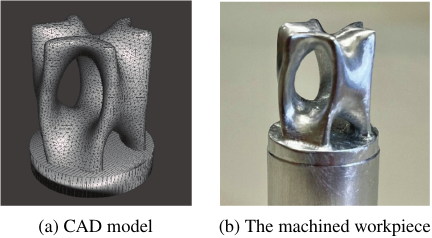
Fig. 19. Product model and machined result in Case 2.
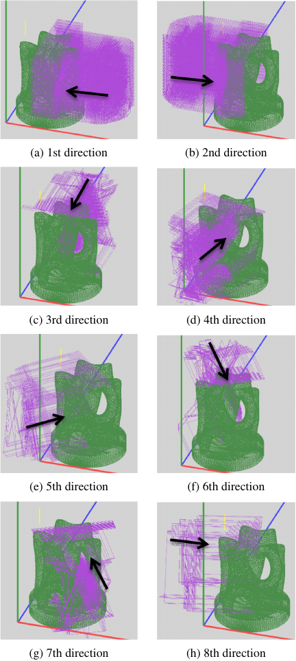
Fig. 20. Roughing tool path with ball end mill in Case 2.
Table 2. Summary of analysis parameters and results for each case study.

Table 2 summarizes the number of triangles in the CAD models, number of indexing orientations automatically determined by the system, and total analysis time for each case study. In both cases, the ray angular interval was set to 15.0°, which was empirically chosen as the balance between the computational load and number of indexing orientations obtained. Preliminary examinations confirmed that a finer angular interval did not significantly change the distribution of feasible orientations but substantially increased the computation time. Nevertheless, for more geometrically complex shapes, adopting a finer interval may improve the robustness of the accessibility evaluation.
The dexel spacing was set as 0.2 mm. A finer spacing improves the fidelity of the machining simulation but significantly increases the computational cost, whereas a coarser spacing (greater than 0.5 mm) results in an insufficient detection of air cuts. Therefore, 0.2 mm was adopted as a practical compromise between accuracy and efficiency.
The analysis was conducted using an Intel Core i9-11900K CPU and NVIDIA GeForce RTX 3080 Ti GPU. Although the above configuration was used to efficiently evaluate the performance, the proposed system did not require such high-end hardware. In practice, this method can also be executed on lower-spec PCs. For example, this configuration has been confirmed to run successfully on a system equipped with a GTX 1650 GPU and a Core i5 CPU. This result indicates that the approach is feasible, even in manufacturing environments with limited computational resources.
In addition, the machining times under the given conditions were approximately 16 h 8 min for Case 1 and 43 h for Case 2.
As shown in Figs. 18 and 20, the proposed method successfully generated feasible and efficient tool paths without collisions or air cuts, even for complex geometries. These results not only confirm the effectiveness of the approach but also underscore its robustness in processing intricate free-form surfaces. Moreover, the relatively short analysis times, even for geometrically complex models, demonstrate the high computational efficiency of the algorithm, making it well-suited for practical deployment in industrial manufacturing environments.
The proposed method is applicable to square and ball end mills. In this study, a general description of roughing performed with a square end mill and finishing with a ball end mill is provided as an example of a typical machining sequence without limiting the applicability of the method. In this case study, a ball end mill was selected as an example because the target geometry consisted of complex free-form surfaces.
Furthermore, in conventional CAM systems, the setup time required to define machining regions, adjust indexing orientations, and perform interference checks strongly depends on the skill of the operator. In contrast, the proposed system automatically accomplished the entire workflow within 5–15 min, as summarized in Table 2. This result demonstrates the advantage of automation in significantly reducing the process planning time while maintaining stable accuracy.
5. Conclusion
This study developed a system to automatically generate indexing orientations and tool paths for 5-axis indexing machining of complex geometries using STL-format CAD models. Furthermore, a shape removal simulation based on the dexel model was implemented to automatically detect air-cut regions and efficiently modify the tool paths. To accelerate processing, parallel computation using a GPU was introduced, resulting in a significant reduction in computation time. This enables the automation of 5-axis machining processes for complex shapes, which traditionally require advanced expertise, thereby allowing flexible and efficient process planning without reliance on skilled operators. This approach is particularly practical for manufacturing environments that require high-precision machining under conditions of high-mix, low-volume production, and short lead-times. However, the analysis time inevitably increases as the model size increases, which is a limitation of the current system. Addressing this limitation, for example, through the further optimization of data structures, will be an important subject for future research. The proposed method depends primarily on geometric data and is therefore, in principle, applicable to various workpiece materials. Differences in material properties can be accommodated by adjusting machining parameters such as the depth of cut and feed rate. Nevertheless, validating the scalability of this approach to larger parts and diverse materials is an important direction for future studies.
Acknowledgments
This study was partially supported by JSPS KAKENHI (Grant Number JP25K01135).
- [1] H. Ueno, “Intelligent technology for machine tools,” Systems, Control and Information, Vol.61, No.3, pp. 107-112, 2017 (in Japanese). https://doi.org/10.11509/isciesci.61.3_107
- [2] K. Nakamoto, K. Shirase, H. Wakamatsu, A. Tsumaya, and E. Arai, “Automatic production planning system to achieve flexible direct machining,” JSME Int. J. Series C, Vol.47, No.1, pp. 136-143, 2004. https://doi.org/10.1299/jsmec.47.136
- [3] Y. Woo, E. Wang, Y. S. Kim, and H. M. Rho, “A hybrid feature recognizer for machining process planning systems,” CIRP Annals, Vol.54, Issue 1, pp. 397-400, 2005. https://doi.org/10.1016/S0007-8506(07)60131-0
- [4] L. Wang, M. Holm, and G. Adamson, “Embedding a process plan in function blocks for adaptive machining,” CIRP Annals, Vol.59, Issue 1, pp. 433-436, 2010. https://doi.org/10.1016/j.cirp.2010.03.144
- [5] A. Ueno and K. Nakamoto, “Proposal of machining features for CAPP system for multi-tasking machine tools,” Trans. of the JSME, Vol.81, No.825, Article No.15-00108, 2015 (in Japanese). https://doi.org/10.1299/transjsme.15-00108
- [6] H. Sakurai, “Volume decomposition and feature recognition: Part 1–Polyhedral objects,” Computer-Aided Design, Vol.27, Issue 11, pp. 833-843, 1995. https://doi.org/10.1016/0010-4485(95)00007-0
- [7] H. Sakurai and P. Dave, “Volume decomposition and feature recognition, part II: Curved objects,” Computer-Aided Design, Vol.28, Issues 6–7, pp. 519-537, 1996. https://doi.org/10.1016/0010-4485(95)00067-4
- [8] E. Morinaga, M. Yamada, H. Wakamatsu, and E. Arai, “Flexible process planning method for milling,” Int. J. Automation Technol., Vol.5, No.5, pp. 700-707, 2011. https://doi.org/10.20965/ijat.2011.p0700
- [9] E. Morinaga, T. Hara, H. Joko, H. Wakamatsu, and E. Arai, “Improvement of computational efficiency in flexible computer-aided process planning,” Int. J. Automation Technol., Vol.8, No.3, pp. 396-405, 2014. https://doi.org/10.20965/ijat.2014.p0396
- [10] K. Okamoto and K. Morishige, “C-space-based toolpath generation for five-axis controlled machining with special tools,” Int. J. Automation Technol., Vol.18, No.5, pp. 679-687, 2024. https://doi.org/10.20965/ijat.2024.p0679
- [11] C.-S. Jun, Y.-S. Lee, and K. Cha, “Configuration-space searching and optimizing tool orientations for 5-axis machining,” Proc. of ASME 2002 Int. Mechanical Engineering Congress and Exposition, pp. 117-127, 2002. https://doi.org/10.1115/IMECE2002-33598
- [12] C.-S. Jun, K. Cha, and Y.-S. Lee, “Optimizing tool orientations for 5-axis machining by configuration-space search method,” Computer-Aided Design, Vol.35, No.6, pp. 549-566, 2003. https://doi.org/10.1016/S0010-4485(02)00077-5
- [13] Z. Mi, C.-M. Yuan, X. Ma, and L.-Y. Shen, “Tool orientation optimization for 5-axis machining with C-space method,” The Int. J. of Advanced Manufacturing Technology, Vol.88, pp. 1243-1255, 2017. https://doi.org/10.1007/s00170-016-8849-0
- [14] Z. Lin, J. Fu, H. Shen, and W. Gan, “Non-singular tool path planning by translating tool orientations in C-space,” The Int. J. of Advanced Manufacturing Technology, Vol.71, pp. 1835-1848, 2014. https://doi.org/10.1007/s00170-014-5629-6
- [15] T. Kanda and K. Morishige, “Tool path generation for five-axis controlled machining with consideration of structural interference,” Int. J. Automation Technol., Vol.6, No.6, pp. 710-716, 2012. https://doi.org/10.20965/ijat.2012.p0710
- [16] J.-N. Lee and R.-S. Lee, “Interference-free toolpath generation using enveloping element for five-axis machining of spatial cam,” J. of Materials Processing Technology, Vols.187-188, pp. 10-13, 2007. https://doi.org/10.1016/j.jmatprotec.2006.11.200
- [17] N. Wang and K. Tang, “Automatic generation of gouge-free and angular-velocity-compliant five-axis toolpath,” Computer-Aided Design, Vol.39, Issue 10, pp. 841-852, 2007. https://doi.org/10.1016/j.cad.2007.04.003
- [18] T. Umehara, K. Teramoto, T. Ishida, and Y. Takeuchi, “Tool posture determination for 5-axis control machining by area division method,” JSME Int. J. Ser. C, Vol.49, Issue 1, pp. 35-42, 2006. https://doi.org/10.1299/jsmec.49.35
- [19] S. N. Grigoriev, A. A. Kutin, and V. V. Pirogov, “Advanced method of NC programming for 5-axis machining,” Procedia CIRP, Vol.1, pp. 102-107, 2012. https://doi.org/10.1016/j.procir.2012.04.016
- [20] M. Inui, S. Nagano, and N. Umezu, “Radial ray representation for fast analysis of optimal cutting direction in 3+2 axis milling,” Proc. Int. Symp. on Flexible Automation, pp. 88-95, 2018. https://doi.org/10.11509/isfa.2018.88
- [21] M. Inui, S. Taguchi, and N. Umezu, “Graphical assistance for determining cutter axis directions in 3+2-axis machining,” Computer-Aided Design & Applications, Vol.20, No.4, pp. 689-703, 2023. https://doi.org/10.14733/cadaps.2023.689-703
- [22] T. Kishinami, “Data exchange and data sharing,” J. of the Japan Society of Precision Engineering, Vol.75, No.1, pp. 48-49, 2009. (in Japanese) https://doi.org/10.2493/jjspe.75.48
- [23] Y. Yamada, T. Okita, and Y. Kuwano, “Indexing 5-axis machining process design support system shortening die fabrication lead time,” Key Engineering Materials, Vols.523-524, pp. 392-397, 2012. https://doi.org/10.4028/www.scientific.net/KEM.523-524.392
- [24] J. Ruan and X. Zhou, “An optimizing tool orientation method for positional 5-axis machining,” 2011 2nd Int. Conf. on Mechanic Automation and Control Engineering, pp. 5561-5564, 2011. https://doi.org/10.1109/MACE.2011.5988286
- [25] I. Nishida, E. Yamada, and H. Nakatsuji, “Automated process planning system for machining injection molding dies using CAD models of product shapes in STL format,” Int. J. Automation Technol., Vol.17, No.6, pp. 619-626, 2023. https://doi.org/10.20965/ijat.2023.p0619
- [26] M. Inui, T. Sakurai, and N. Umezu, “Data conversion technology between triple dexel model and polygonal model,” J. of the Japan Society for Precision Engineering, Vol.76, No.2, pp. 226-231, 2010 (in Japanese). https://doi.org/10.2493/jjspe.76.226
- [27] M. Inui and N. Umezu, “Contour-type cutter path computation using ultra-high-resolution dexel model,” Computer-Aided Design and Applications, Vol.17, No.3, pp. 621-638, 2020. https://doi.org/10.14733/cadaps.2020.621-638
- [28] M. Inui, “Visualization of machined shape in 3+2-axis machining by Triple-Dexel Integration of Multiple Z-Map Models,” Proc. of the 18th Int. Conf. on Manufacturing Research, pp. 413-418, 2021.
This article is published under a Creative Commons Attribution-NoDerivatives 4.0 Internationa License.