Research Paper:
Shipment Forecasting for Yellowtail Aquaculture Using Monte Carlo Simulation: A Scenario Analysis on the Utilization of Hatchery-Produced Juveniles
Yuki Kimura*,† and Tomomi Nonaka**

*Graduate School of Creative Science and Engineering, Waseda University
3-4-1 Okubo, Shinjuku-ku, Tokyo 169-8555, Japan
†Corresponding author
**School of Creative Science and Engineering, Waseda University
Tokyo, Japan

In Japan’s key yellowtail (buri) aquaculture industry, the increasing exports are contrasted with the production instability caused by declining producers and a reliance on wild juveniles with long, unpredictable lead times. This study addresses these challenges by proposing a production management approach that utilizes hatchery-produced juveniles with controllable, twice-yearly spawning schedules (spring and autumn) to improve the efficiency and predictability. A Monte Carlo simulation using probability distributions determined by the Anderson–Darling test was employed to analyze the shipment patterns and revenue under three pricing scenarios: high-seasonal, moderate, and size-differentiated. The results demonstrate that an increase in the number of spawning seasons distributes shipments more uniformly. This results in a stable year-round supply. The approach can significantly increase the annual revenue, particularly in the high-seasonal price scenario. Conversely, although the differentiated pricing model marginally reduces the total revenue, it significantly mitigates seasonal sales fluctuations. Thus, it provides enhanced stability for producers. To conclude, this study shows that utilizing hatchery-produced juveniles enhances the economic resilience and operational sustainability. This shift toward a more controlled and efficient system aligns with the core sustainability principles. The methodology also provides an adaptable model for other aquaculture sectors. Future work should incorporate the market demand and environmental variables to develop more comprehensive decision-making tools.
1. Introduction
1.1. Research Background
Yellowtail (buri) is a major species in Japan’s marine aquaculture industry. It has been designated as a priority item in the government’s “Export Expansion Implementation Strategy” 1. Although the annual production volumes fluctuate owing to natural factors, both export volume and export value have shown an upward trend in recent years 2. Meanwhile, the number of yellowtail aquaculture producers has been reducing 2. This is particularly so among sole proprietors, whose numbers reduced from 642 in 2003 to 354 in 2013 (representing a nearly 50% decrease) 3. The factors contributing to this reduction include Japan’s contracting labor force, high rearing costs, and the difficulty of securing stable profits owing to the impacts of natural phenomena. However, with the growing demand owing to an expanding overseas market in addition to the domestic needs, there is a call to expand production beyond the current levels. This makes it imperative to increase the output per producer and improve the overall production efficiency.
Traditionally, yellowtail aquaculture involves capturing wild-caught juveniles and rearing these for approximately two years before being shipped. Compared with conventional manufacturing, this process involves a long lead time. This hinders shipment forecasting and production management. Furthermore, there is a significant risk of mass mortality owing to disease outbreaks or red tides. To address these challenges, the research on hatchery-produced juveniles has advanced in recent years. This has resulted in the development of fish with controllable growth rates and spawning schedules 4.
Mushiake 4 reared hatchery-produced juveniles to a size comparable to that of their wild-caught counterparts by controlling the water temperature and photoperiod. It has also been demonstrated that the use of hatchery-produced juveniles enables a year-round supply of yellowtail with stable quality and further improves the productivity through selective breeding 5. Kurose Suisan Co., Ltd. 5 established an artificial seed production technology that addresses the entire process from egg collection to juvenile rearing. It enables egg collection and seed production up to five times per year. Moreover, the use of artificial seedlings has enabled the selection of lineages with superior genetic traits, thereby allowing for the preferential production of healthy, fast-growing yellowtail 5. However, the research on shipment forecasting and the production management indicators for yellowtail aquaculture that specifically account for the unique characteristics of hatchery-produced juveniles is limited. If the effectiveness of yellowtail aquaculture using artificial breeding technology can be clarified from the perspectives of shipment volume and production management, the use of hatchery-produced juveniles (which are currently limited to a small number of producers) is likely to spread nationwide and contribute to increasing the overall production of farmed yellowtails.
1.2. Research Objective
This study aimed to develop a growth flowchart and define production management indicators for yellowtail aquaculture. The appropriate probability distributions for these indicators were identified using the Anderson–Darling (A-D) test, followed by shipment forecasting through a Monte Carlo simulation based on predefined scenarios. In the scenario analysis, we evaluated the effectiveness of hatchery-produced juveniles by simulating an increase in the number of peak shipment periods enabled by manipulating their spawning schedules.
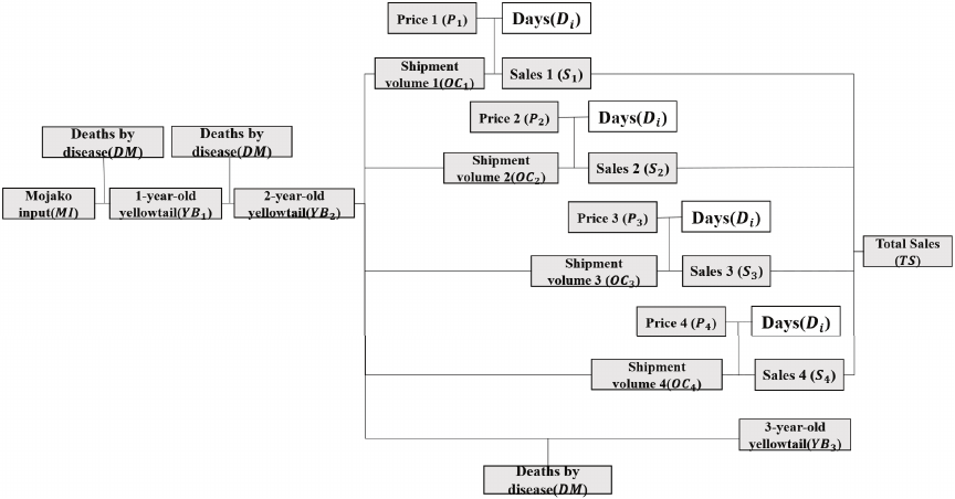
Fig. 1. Growth flow model for farmed yellowtail.
2. Simulation Method
2.1. Previous Research
Production management indicators have been widely studied and applied in the manufacturing industry. Therein, processes are typically deterministic, repeatable, and governed by highly controllable conditions 6,7. In contrast, aquaculture involves biological systems subject to environmental variability, individual growth differences, and uncontrollable external factors such as the water temperature and weather. These characteristics require different production management approaches.
In the agricultural domain, Unn et al. 8 developed a set of production indicators for pig farming and conducted shipment forecasting using Monte Carlo simulations. Their indicators included 13 related to breeding and 10 related to fattening, based on a year of empirical data collected from pig farms. For the probability distributions applied in the Monte Carlo simulations, they fitted 21 types and conducted the A-D test. They selected the distribution with the lowest test statistic provided it was at most 1.5. They performed 1,000 simulation trials. The study 8 demonstrated that most of the probability distributions were sufficiently appropriate based on the A-D test results and that the Monte Carlo simulations could function effectively when using accurately fitted distributions. Similarly, Sugimura et al. 9 conducted a study on demand forecasting for wholesale markets of lettuces to support production planning in plant factories. Although the target product differs, their study also emphasizes the importance of forecasting models in production planning for biological systems. In the present study, we adapted and extended the production indicators developed in 8 to the context of yellowtail aquaculture.
2.2. Growth Process in Yellowtail Aquaculture
Yellowtail juveniles are known as mojako. These are captured from the sea and placed in net cages. Herein, these grow to approximately 1 kg by December of the same year 10. The following year, larger individuals weigh approximately 2 kg 10. In the autumn, these typically grow to approximately 3.5 kg. At this point, shipments begin 10. During this period, the fat content of fish increases significantly. This makes it the peak season for farmed yellowtail 10. The primary shipping season is December–February. In this period, large volumes of yellowtail are shipped daily 10. Even after the peak passes, farming continues to ship large yellowtails for overseas markets. However, from the third year onward, the fish enter a maturation phase and become mature yellowtails with reduced body fat and weight. Therefore, continuing to farm them into their third year and beyond involves a significant risk for producers 10.
2.3. Growth Flow Model and Data Used
Figure 1 shows the growth model developed based on the actual growth process in yellowtail aquaculture described in Section 2.2. In this study, all the components shown in Fig. 1 (except for days) were defined as production management indicators. This model progresses from left to right. Thus, it represents the flow of time and shows the computational structure for calculating the sales value.
The number of mojako inputs (\(\textit{MI}\)) is based on the estimated number of juvenile fish stocked from 11. Meanwhile, the number of yellowtail deaths by disease (\(\textit{DM}\)) uses the fish disease damage ratio from 12. It should be noted that the damage ratio to production value owing to fish disease was directly applied as the damage ratio to the number of individual fish. The number of one-year-old yellowtail (\(\textit{YB}_1\)) and two-year-old yellowtail (\(\textit{YB}_2\)) were estimated by applying the disease mortality rate to the initial number of mojako inputs. The number of three-year-old yellowtail (\(\textit{YB}_3\)) was estimated using Eq. \(\eqref{eq:1}\). Here, \(\alpha\) represents the age-class composition of the shipped fish 11. Age-class composition is defined as “the ratio determined by maximizing the correlation coefficient between the actual production volume (production statistics) and the number of juveniles stocked in the previous and second-previous years” 11. In this study, \(\alpha\) was set to 0.28. For the shipment volume (\(\textit{OC}_i\)) and price (\(P_i\)), the transaction volume (\(A_j\)) for farmed yellowtails in the Osaka Market from April 2003 to October 2024 (sourced from Jiji Press’s “Jiji Fishery News” 13) was used. Note that in this paper, the subscript “\(i\)” refers to the four periods described subsequently, and “\(j\)” refers to the time-series serial number in the reference data 13. The long-term data on farmed yellowtail required for this study are available only for the Toyosu and Osaka Markets. A comparison of the data of the two markets revealed that those for the Toyosu Market have scattered missing values. Therefore, the transaction volume from the Osaka Market (which was recorded more continuously and comprehensively) was used to estimate the national shipment volume. To account for the differences in the body size of yellowtail depending on the shipping season and to consider the peak season, the shipment volume and price data were divided into four periods corresponding to the four seasons. In accordance with 14, the year is divided into four periods: Period 1 is spring (March–May), Period 2 is summer (June–August), Period 3 is autumn (September–November), and Period 4 is winter (December–February; corresponds to the conventional peak season). The shipment volume is adjusted to the national scale by Eq. \(\eqref{eq:2}\). The multiplier (\(\beta\)) used for this adjustment was calculated from the average annual transaction volume in the Osaka Market and the average national production volume from reference 11 for 2004–2023. The average for the Osaka Market was 488,916 kg, and the average national production was 92,684,211 kg. Therefore, \(\beta\) was set to 190. The sales value (\(S_i\)) was calculated using Eq. \(\eqref{eq:3}\), and the total sales value (\(\textit{TS}\)) was calculated using Eq. \(\eqref{eq:4}\). \(D_i\) represents the number of days. In this study, it was set to a constant value of 90 days as a prerequisite for the analysis. Red tides were excluded from the study.
2.4. Distribution Estimation Using the Anderson–Darling Test (A-D Test)
Following the analysis method of Unn et al. 8, we determined the best-fit distribution by fitting 21 types of probability distributions to each indicator and performing an A-D test. The probability distribution developed from the source data described in Section 2.3 is defined as the “assumed distribution.” The probability distribution developed using this assumed distribution is defined as the “predictive distribution.”
The other commonly used goodness-of-fit tests include the Kolmogorov–Smirnov (K-S) and Shapiro–Wilk tests. However, the Shapiro–Wilk test is primarily used for testing normality, and the K-S test emphasizes the fit in the central part of the distribution. In forecasting shipments for aquaculture, it is necessary to consider the standard trends and extreme values generated by uncertain factors such as weather and disease. Although pig farming studied by Unn et al. 8 also has a high uncertainty, we considered it even more critical to emphasize the extreme values for yellowtail aquaculture in this study. This was because yellowtail aquaculture involves a significant risk (although it may be infrequent) of shipments reducing to zero for a period owing to a red tide event. Unlike the K-S test and others, the A-D test can assess the goodness-of-fit at the ends of the distribution (known as the “tails”) with sensitivity equal to that in other parts 15. In this study, we considered the A-D test to be the most appropriate because it evaluates tails with equal weight as the center rather than focusing only on the center.
The following continuous distributions were used: normal, triangular, uniform, exponential, lognormal, beta, gamma, logistic, Student’s \(t\)-test, Weibull test, minimum extreme value, maximum extreme value, and the Pareto test. The following discrete distributions were used: binomial, discrete uniform, geometric, hypergeometric, negative binomial, Poisson’s, and yes–no. Additionally, a custom distribution 15, which is a combination of discrete and continuous distributions, was used.
If the data for each indicator followed each of the 21 probability distributions, we generated random numbers 10 times for each type of distribution and performed the A-D test. The test value was the average of the results from 10 trials. The selection criterion for the best-fit distribution was that it should have the lowest average test statistic among those that fit at the 5% significance level.
2.5. Scenario Settings
A scenario analysis was conducted to evaluate the impact of altering the spawning season and thereby increasing the number of peak seasons. In this study, we assumed that spawning occurs twice a year (in spring and autumn) rather than once a year (in spring). Furthermore, we established the following three pricing scenarios. The total shipment volume was assumed to remain constant across all the scenarios.
Scenario 1:The prices are set at conventional market rates corresponding to the four seasons without considering the different spawning schedules.
Scenario 2:The prices for the new peak seasons (summer and winter) are set at the high market prices of the conventional peak season (winter).
Scenario 3:The prices are differentiated based on the differences in body size resulting from the different spawning schedules.
In Scenario 1, the spawning schedule of farmed yellowtail is not considered, and a uniform price is applied to all the yellowtails in the market. The seasonal price fluctuations are assumed to be identical to that in the current situation. Thus, a scenario in which only the shipment schedule differs from that in the conventional model is postulated.
In Scenario 2, like Scenario 1, a uniform price is applied to all yellowtails sold. However, the prices for summer and winter (which now serve as peak seasons based on the growth cycle following spawning) are set to the traditional peak (winter) market price.
In Scenario 3, different spawning schedules are considered. The prices are set at two levels to reflect the resulting differences in body size.
In each scenario, the shipment volume for a given season was calculated by summing the volumes from two separate production periods to reflect the effect of staggering spawning schedules over six months. That is, the spring shipment volume is the sum of the volumes in Periods 1 and 3, and the summer shipment volume is the sum of the volumes in Periods 2 and 4.
2.6. Monte Carlo Simulation
A Monte Carlo simulation was performed for the shipment volume and price indicators based on the best-fit distributions determined by the A-D test. Aquaculture is affected significantly by uncontrollable stochastic factors such as the weather and market prices. To evaluate the risks posed by these uncertainties, a Monte Carlo simulation involving random sampling based on the probability distribution of each indicator was determined to be appropriate 15. With the number of trials set to 1000, the simulation forecasted the shipment volume and price for a 90-day period. Next, we calculated the projected sales value. In this analysis, it was assumed that even with a modified spawning season, the total annual number of mojako used for yellowtail aquaculture and the total annual shipment volume would remain unaltered. Therefore, the spring and autumn spawning cohorts were assumed to use half of the conventional total number of mojako. Consequently, half the shipment volume projected by the simulation for each period was used to calculate the sales value. Based on these processes, simulations were performed under identical conditions by applying the settings for each scenario described in Section 2.5, and the mean values and standard deviations were calculated. Furthermore, a paired \(t\)-test was used to verify whether the difference in total sales between the conventional method and each scenario is statistically significant. In this study, a difference was considered statistically significant if the \(p\)-value was less than 0.05 (\(p\) \(<0.05\)).
Table 1. Best-fit distributions.

3. Results
3.1. Determination of Best-Fit Distributions
Table 1 presents the meaning, variance, and results of the A-D test for each production indicator item shown in Fig. 1 This test was conducted using 21 types of probability distributions. The most suitable probability distribution for each indicator was selected based on the test statistic. The results are shown in the column labeled “Best-Fit Distribution.” The results of the A-D test are favorable for all the indicator items.
The characteristics of the distributions selected as the best fit are described below. The normal distribution is a symmetrical “bell-shaped” distribution centered around the mean value. Its variable can adopt any real value. The logistic distribution is also a symmetrical “bell-shaped” distribution. It is extremely close to the normal distribution. Its variable can also adopt any real value. The logistic distribution is characterized by a high kurtosis compared with the normal distribution. The minimum extreme value distribution is one of the extreme value distributions and is asymmetrical. It displays the shape of a long tail extending to the left side (negative side). Its variable range comprises all real numbers. The shape of the Weibull distribution varies flexibly depending on its parameters. Depending on the parameters, a shape like that of an exponential distribution, a bell shape close to normal, or a right-skewed shape can be assumed. The variable range constitutes only positive values. The lognormal distribution is asymmetrical, skewed to the left (0), and displays the shape of a long tail extending to the right (right-skewed). The variable range constitutes only positive values.
3.2. Simulation Results
3.2.1. Price
Table 2 lists the values for each item predicted by the simulation. According to Table 2, the predicted average price for Period 3 was the highest, whereas that for Period 1 was the lowest. The variances were smaller for the relatively low-priced Periods 1 and 2 and larger for the high-priced Periods 3 and 4. The range (the difference between the maximum and minimum values) was larger for Periods 3 and 4 than for Periods 1 and 2. This indicates a higher data dispersion.
Table 2. Monte Carlo simulation results (price).

3.2.2. Shipment Volume
Table 3 lists the values for each item predicted by the simulation. Table 4 presents the projected total shipment volume per period for both conventional method and method with an increased number of peak seasons. As shown in Table 3, the shipment volume in Period 1 was the highest and that in Period 2 was the lowest. Although marginal differences are observed in values other than the mean, these are less significant than those in the price data. Table 4 indicates that with the conventional method, the shipment volume for Period 1 was the highest. Compared with the conventional method, the total shipment volume decreased in Periods 1 and 4 and increased in Periods 2 and 3 when the spawning schedules were staggered by six months to increase the peak seasons. The breakdown column shows that staggering the spawning schedules by six months resulted in equal shipment volumes for the spring/autumn and summer/winter periods.
Table 3. Monte Carlo simulation results (shipment volume).

Table 4. Projected total shipment volume.

3.3. Scenario Analysis
The results for the projected sales value (calculated using the Monte Carlo simulation) were aggregated for each scenario. Tables 5, 6, and 7 show the mean and standard deviation of projected sales for Scenarios 1, 2, and 3, respectively. Table 8 shows the mean and standard deviation of the projected sales value for yellowtail aquaculture with the conventional single annual peak season (designated the Base Scenario). The price and shipment volume for the Base Scenario are described in Section 3.2. The results for each scenario are described in detail in the following subsections.
3.3.1. Scenario 1
The total sales value was projected to be equivalent to that of the Base Scenario. Furthermore, a comparison of sales values by period revealed a seasonal fluctuation like that in the Base Scenario, with lower sales in Periods 1 and 2 and higher sales in Periods 3 and 4.
Table 5. Projected sales value (Scenario 1).

Table 6. Projected sales value (Scenario 2).

Table 7. Projected sales value (Scenario 3).

Table 8. Projected sales value (Base Scenario).

3.3.2. Scenario 2
The sales value was projected to be higher than that in the Base Scenario. It was also projected to yield the highest sales value among the three scenarios. From the sales value by period, the sales for Period 2 were higher than those for the other cases. For the other periods, like the Base Scenario, the sales in Period 1 were low, whereas the sales in Periods 3 and 4 were high.
3.3.3. Scenario 3
The resulting total sales value (mean and standard deviation) was projected to be approximately equivalent to that in the Base Scenario. An examination of the sales value by period revealed that the seasonal fluctuation was less than that in the other cases. This indicates that a more stable sales value could be obtained throughout the year.
The standard deviation of total sales increased in Scenario 2. However, its value in Scenarios 1 and 3 was approximately equivalent to that in the Base Scenario. However, Scenarios 1 and 3 showed small standard deviations in all the four periods compared with the Base Scenario.
4. Discussion
4.1. The Fitted Distributions from the A-D Test
Based on Table 1, the fitted distribution for each indicator item is as follows:
The fitted distribution for the mojako input is a logistic distribution. The number of mojako inputs is influenced by the annual ocean currents and weather. Therefore, it is natural to assume a symmetrical shape around the mean value. In addition, “bumper catch” and “poor catch” years occur frequently. This is considered to result in a high kurtosis compared with a normal distribution. Therefore, a logistic distribution was fitted. One-year-old yellowtail had the minimum extreme value distribution. This indicator represents the number of fish that survived for one year from the mojako stage. From the fitted distribution, it can be stated that in most years, many mojako survived. However, it is also conceivable that a massive die-off from disease or red tide could have occurred, thereby causing the survival count to reduce abruptly. The minimum extreme value distribution was fitted considering the risk. The two- and three-year-old yellowtail exhibited Weibull distributions. The mortality rate of fish is not constant and is considered to vary with age. The Weibull distribution is used to model phenomena in which the probability of occurrence varies over time. Therefore, it is considered that this distribution was fitted.
Shipment volumes in Periods 1 and 4 exhibit Weibull distributions. Period 1 is the decreasing period after the peak. Period 4 is the peak season. Neither of these periods has a stable mean value. Rather, abrupt increases and decreases occur daily. The Weibull distribution was fitted because it can flexibly represent this phenomenon (where the probability varies over time). Shipment volume in Period 2 exhibits a logistic distribution. Period 2 is the off-season for yellowtail. Therefore, a stable distribution around the mean value is likely. However, it is also conceivable that values deviating from the mean could occur because of factors such as the weather. Therefore, it is considered that a logistic distribution would fit, rather than a normal distribution. Shipment volume in Period 3 exhibits a lognormal distribution. This period occurs before the peak season, and the shipment volume is not significantly high. However, as the peak season approaches, the likelihood of large-scale shipments is considered. Therefore, the lognormal distribution (which has a long right tail) was fitted.
Price in Period 1 exhibits a logistic distribution. It is a stable price near the mean value. Additionally, like the other indicators that fit the logistic distribution, it is considered to fit this distribution because of price fluctuations (both upward and downward) from uncertain factors. Price in Period 2 exhibits a lognormal distribution. This is because although the price has a lower limit of JPY 0, abrupt price spikes owing to unforeseen demand are likely even in the off-season. This asymmetrical shape is considered to have resulted in the fit. Prices in Periods 3 and 4 exhibits a minimum extreme value distribution. This indicates that unlike price in Period 2 , the prices are stable at a high level on most days. However, a price crash owing to oversupply is likely, such as concentrated shipments. A minimum extreme value distribution was fitted to express this risk.
Period 1: Sales are logistically distributed. Period 1 is the off-season. Similar to price in Period 1 , it is considered to have a stable “bell shape” around a mean value. However, the risk of infrequent sales fluctuations is conceivable. Therefore, the logistic distribution is considered to have fitted, rather than a normal distribution. Sales in Period 2 exhibits a lognormal distribution. This distribution has a long right tail, which matches the sales reality of the off-season Period 2. That is, the sales have a lower limit of JPY 0 and are stable at a low level on most days. However, abrupt spikes in sales are likely. Therefore, a lognormal distribution was fitted. Sales in Period 3 displays a normal distribution. In this period, sales prices are relatively stable as they immediately precede the peak season (Period 4). Furthermore, it is considered that various random factors, such as weather and demand, cancel each other out. As a result of the central limit theorem taking effect, the distribution converges to the most stable, symmetrical “bell shape.” Sales in Period 4 follows a Weibull distribution. Although Period 4 is the peak season, it includes both “increase toward the peak” and “decrease after the peak.” Therefore, it is a phenomenon where the probability varies over time, and it is considered that the Weibull distribution was fitted.
Finally, total sales displays a normal distribution. This is a manifestation of the central limit theorem. Even if the component distributions are different, “summing” many of these would approach a normal distribution. Because total sales is the sum of sales from each period, it is considered that the central limit theorem takes effect and fits the normal distribution.
4.2. Shipment Volume
This section examines the shipment volume under the Base Scenario. Specifically, we investigated how staggered spawning seasons affect shipment patterns and evaluated the stability of shipment quantities throughout the year. From the results in Section 3.2.2, staggering the spawning season to increase the number of peak seasons resulted in equal shipment volumes for the spring–autumn and summer–winter periods. In this analysis, the shipment volumes were held constant across all the cases to isolate and examine the impact of price fluctuations. This explains why these numbers were identical. However, because the simulation was based on predictive distributions derived from actual data, it is conceivable that even if the shipment volume were simulated in each trial, the volumes for the spring/autumn and summer/winter periods would have remained similar. That is, if the spawning season is staggered strategically to create multiple peak periods, the shipment pattern is likely to shift toward a half-year cycle with seasonal fluctuations. Furthermore, as shown in Table 4, the overall annual fluctuation in the shipment volume is smaller than that for the conventional method. This indicates that shipping a stable quantity of yellowtail throughout the year would become feasible.
4.3. Scenario 1
From the results in Section 3.3.1, the projected sales value in Scenario 1 was almost equivalent to that in the Base Scenario. From the results of the paired \(t\)-test described in Section 2.6, the difference in total sales value between Scenario 1 and the Base Scenario was not statistically significant (\(p=0.140\)). Thus, if the pricing structure remains identical to that in the conventional method, an increase in the number of peak seasons has a limited impact on the total sales value.
4.4. Scenario 2
From the results in Section 3.3.2, the projected sales values in Scenario 2 were the highest. Additionally, the t-test results were statistically significant (\(p < 0.001\)). Furthermore, the projected sales values for Periods 1, 3, and 4 were comparable to those for the conventional method, whereas the value for Period 2 increased significantly compared with the other scenarios. It is considered that this increase in Period 2 sales value had a major impact on the increase in total sales value. This significant increase in sales value in Period 2 is likely to have resulted from the use of the conventional peak season price (the price in Period 4) in the calculation. Scenario 2 was the only scenario in which all yellowtails were priced at the peak season rate during the newly added summer peak season (created by staggering the spawning time) regardless of the fish body size. According to Table 2, the average price in Period 4 was higher than that in Period 2 by approximately JPY 230. That is, an increase in the number of peak seasons during which yellowtail can be sold at a relatively high price can cause an increase in sales value.
4.5. Scenario 3
From the results in Section 3.3.3, the total sales value was identical to that of the Base Scenario. In addition, the t-test results clarified that there was no statistically significant difference in total sales value between the Base Scenario and Scenario 3 (\(p=0.913\)). However, it was projected that seasonal fluctuations in sales value would be suppressed, thereby enabling the achievement of stable sales values throughout the year. From the standard deviation for each period, Scenario 3 showed a significant decrease compared with the Base Scenario. This is likely to have resulted from the six-month staggering of the spawning season and the establishment of two price tiers based on individual body sizes in Scenario 3. Staggering the spawning season suppresses the seasonal fluctuations in the shipment volume. In addition, setting two price tiers implied that the relatively low prices in Periods 1 and 2 were used concurrently with the high prices in Periods 3 and 4. That is, it is considered that this six-month staggering served to even out seasonal fluctuations. Therefore, Scenario 3 is regarded to have demonstrated the feasibility of stabilizing only the risk of seasonal fluctuations without reducing the total annual sales value, unlike conventional yellowtail aquaculture (which experiences seasonal fluctuations in sales). It is a valid option that could stabilize producers’ business management.
5. Conclusion
In this study, we employed Monte Carlo simulations to forecast shipment volumes and pricing outcomes in yellowtail aquaculture using hatchery-produced juveniles with staggered spawning schedules. A growth flow model and a set of production management indicators were identified using the A-D test. The scenario analysis results show an increase in shipment volume during conventional low-volume periods. This indicates the potential for high annual sales compared with the conventional method. Furthermore, by strategically adjusting spawning schedules and pricing, it is feasible to achieve a stable annual sales value throughout the year.
As a future challenge, it is necessary to consider additional factors such as the demand trends and the impact of natural phenomena. This study used only supply-side data and excluded considerations such as the demand fluctuations owing to peak seasons. Environmental factors such as red tides and global warming were excluded from the analysis. Therefore, further research based on more realistic and comprehensive hypotheses incorporating these factors is necessary. Furthermore, expanding the perspective of this study to the micro level could also be considered. This study conducted shipment forecasting from a macro-level perspective by targeting Japan as a whole and demonstrated the potential to increase shipment volume and achieve stable annual sales for the entire yellowtail aquaculture industry. Nonetheless, the implications for production management at the individual enterprise level during the expanded peak seasons have not been examined sufficiently. Therefore, research from a micro-level perspective using production management data from individual enterprises is necessary.
- [1] Ministry of Agriculture, Forestry and Fisheries, “Export expansion strategy for agriculture, forestry, and fishery products and food—For the transition to market-in exports,” Materials for the Ministerial Council on Import Country Regulations for Export Expansion of Agriculture, Forestry, and Fishery Products and Food, 2023 (in Japanese).
- [2] Fisheries Agency, “Recent state of the aquaculture industry,” Document 1, 2024 (in Japanese).
- [3] Development Bank of Japan Inc., “Southern Kyushu fisheries survey: growth strategy for yellowtail aquaculture,” Development Bank of Japan Inc., 2016.
- [4] K. Mushiake, “Technology of spawning period regulation and egg quality evaluation method,” Bulletin of the Institute for Marine Biological Resources, Fukuyama University, Vol.18, pp. 31-35, 2008 (in Japanese).
- [5] Kurose Suisan Co., Ltd., “Corporate news: Aiming for a new form of yellowtail aquaculture,” The Japanese Society of Fisheries Science, Vol.86, No.3, pp. 237-238, 2020 (in Japanese). https://doi.org/10.2331/suisan.WA2706
- [6] N. Ueno, M. Kawasaki, and H. Okuhara, “Mass customization production planning system by advance demand information based on unfulfilled-order-rate,” J. of the Institute of Systems, Control and Information Engineers, Vol.23, No.7, pp. 147-156, 2010 (in Japanese). https://doi.org/10.5687/iscie.23.147
- [7] H. Fukui and F. Hashimoto, “A study on the method for due-date assignment in case of varying the shop load levels,” J. of Japan Industrial Management Association, Vol.46, No.4, pp. 242-247, 1995 (in Japanese). https://doi.org/10.11221/jimapre.46.4_242
- [8] S. Unn, T. Sugimoto, A. Kurokawa, H. Takahashi, and K. Akachi, “A case study of shipment pig prediction and risk analysis by Monte Carlo method,” J. of the Japanese Agricultural Systems Society, Vol.25, No.3, pp. 157-165, 2009 (in Japanese). https://doi.org/10.14962/jass.25.3_157
- [9] N. Sugimura, N. Q. Thinh, S. Kohama, Y. Fukui, and K. Iwamura, “A study on demand forecasting of wholesale markets of lettuces for production planning in plant factories,” Int. J. Automation Technol., Vol.16, No.2, pp. 218-229, 2022. https://doi.org/10.20965/ijat.2022.p0218
- [10] Japan Fisheries Research and Education Agency (FRA), “Special feature: aiming for the spread of ‘artificial seedlings of yellowtail’,” FRA NEWS, Vol.70, 2022 (in Japanese).
- [11] Fisheries Agency, “Regarding trends in the production and export of farmed yellowtail,” Farmed Fish Supply and Demand Review Meeting, Document 1, pp. 1-5, 2024 (in Japanese).
- [12] Ministry of Agriculture, Forestry and Fisheries, “The current situation surrounding fish diseases,” 1st Fish Disease Countermeasures Promotion Council, Document 2, 2019 (in Japanese).
- [13] Jiji Press Ltd., “Jiji Suisan Joho (Jiji Fisheries Information) homepage,” 2025. https://suisan.jiji.com/info/ [Accessed July 25, 2025]
- [14] Japan Meteorological Agency, “Forecast terminology: ‘Terms related to time’,” (in Japanese). https://www.jma.go.jp/jma/kishou/know/yougo_hp/toki.html [Accessed July 25, 2025]
- [15] D. Vose, “Introduction to risk analysis: from basics to practice,” T. Hasegawa and M. Tsutsumi (Trans.), Keiso Shobo, 2003 (in Japanese).
This article is published under a Creative Commons Attribution-NoDerivatives 4.0 Internationa License.