Research Paper:
Energy Consumption-Oriented Process Design Based on Specific Energy-Consumption Model
Kazuki Shimomoto†, Masaki Nakamura, and Tetsuo Samukawa

Faculty of Science and Engineering, Setsunan University
17-8 Ikeda-nakamachi, Neyagawa, Osaka 572-8508, Japan
†Corresponding author

Reducing the energy needed for the machining processes used in manufacturing is a concrete step toward achieving a green transformation (GX). In this study, we investigated the use of a three-axis vertical machining center to drill and end mill a workpiece and evaluated the effects of different process designs and machining conditions on the energy efficiency. Evaluations of the energy consumption, which included the energy consumed during machining as well as that consumed for material mounting and tool changes, showed that the optimal process differed depending on the production volume. Furthermore, the evaluation results mostly agreed with the measurements. The proposed method can be implemented using numerical-control-program simulation data based on computer-aided manufacturing software. Thus, it is a practical energy-saving technology that does not require additional equipment. The proposed method is expected to contribute to the realization of sustainable production activities that promote a GX at manufacturing sites.
1. Introduction
To realize a carbon-neutral society, it is important to conserve energy, improve energy efficiency, and reduce the environmental load in the manufacturing industry. Energy conservation has been promoted by improving or reducing the weight of machine tools, which are the major devices used in manufacturing 1,2,3,4. However, the introduction of new machines imposes an economic burden; therefore, this is not always a viable option. It is also possible to conserve energy by setting suitable cutting conditions using existing equipment 5,6,7. The application of energy-conservation technology in the operational planning stage of a system comprising individual machines is becoming increasingly important. One example is production planning, which considers energy and environmental loads 8,9,10. The evaluation and modeling of the cutting force, energy consumption, and environmental load discharge are important for technology-supporting planning 11,14,15,16,12,13. Energy and environmental loads are used as evaluation indices in the process-design stage 17,18. Thus, studies to reduce the energy consumption and environmental impact are being actively conducted in various areas. However, discussions on process-design methods that consider energy consumption at the production planning stage remain inadequate. Therefore, in this study, we investigated a process-design method that makes it possible to achieve energy conservation using an existing specific energy consumption model targeting the portion of the manufacturing process that involves drilling and end milling. We verified that it is possible to determine the optimal tool configuration and process depending on the production volume using a process design based on computer-aided manufacturing (CAM) and predictions based on a specific energy-consumption model. First, we measured the energy consumption during machining, idling, and axis movement using a simple cutting experiment. The energy consumption during machining could be analyzed from the material removal rate and specific energy consumption and formed the basis for constructing a specific energy-consumption model. Next, we used CAM to produce multiple machining processes with different tool configurations or cutting conditions for machining the same part. The model was used to evaluate the total energy consumed in each case, including the setup time. We compared the results of the evaluated total energy consumption, identified the processes that would make it possible to conserve energy, and demonstrated the feasibility of the specific energy-consumption model. In addition, we evaluated the productivity and economic costs of the different modes and obtained data that can assist in a process-design approach oriented toward multipurpose optimization.
2. Previous Study
2.1. Energy-Saving Process Design
Although the optimization of productivity and economic costs has been the goal of process design in the past, studies that include energy and environmental loads as evaluation indices are becoming increasingly important. Oda et al. 17 compared the amounts of energy consumed during turning, facing, and end milling using a multifunctional machine tool, and identified the machining processes that should be prioritized. Fysikopoulos et al. 18 compared the energy efficiencies of drilling and abrasive water-jet machining in drilling operations. It is possible to compare the energy efficiencies of different machines or conditions used to execute a given machining process by analyzing the energy consumed per unit of material removed (specific energy consumption). Gutowski et al. presented the specific energy-consumption values of machining, grinding, and electrical discharge machining (EDM), and showed that processing methods with high material-removal rates are preferable from the standpoint of energy saving 19. Kara and Li showed that, in turning, the use of cutting conditions with high material removal rates led to energy conservation 20. These studies identified methods that resulted in greater energy conservation in terms of individual machining processes. However, the effects of tool selection or differences in production volume at the actual process-design stage on the total energy consumption have not been sufficiently assessed. Therefore, in this study, we investigated a process design that considered the setup time required for tool mounting or exchange, along with the accompanying energy consumption, with the goal of achieving a process design that considers energy more practically.
2.2. Specific Energy-Consumption and Power-Consumption Models
To evaluate the energy consumption in advance, we employed the processing time and material removal rate computed from a CAM simulation, along with a specific energy-consumption model that allowed us to predict the energy consumption. If \(V\) [mm\(^3\)] is the volume removed during machining time interval \(t_{\mathit{cut}}\) [s], material removal rate \(v_m\) [mm\(^3\)/s] can be expressed as follows:
The specific energy consumption, \(c\) [J/mm\(^3\)], can be derived by dividing the total energy consumption, obtained from the machining power consumption \(P_{\mathit{cut}, i}\) [W], by \(V\) [mm\(^3\)], as follows:
We considered predicting \(c\) using a specific-energy-consumption model. While it is possible to make an assessment using the representative models of Gutowski et al. 19 or Kara and Li 20, or their derivatives (see for instance 21,22,23,24), in this study, we employed a model proposed by the authors in a previous study 25. We proposed a regression model in which the relationship between \(c\) and \(v_m\) is expressed by a power law, as follows:
Our previous study 26 showed that this power consumption model exhibits high prediction accuracy for the energy consumption and is highly versatile.
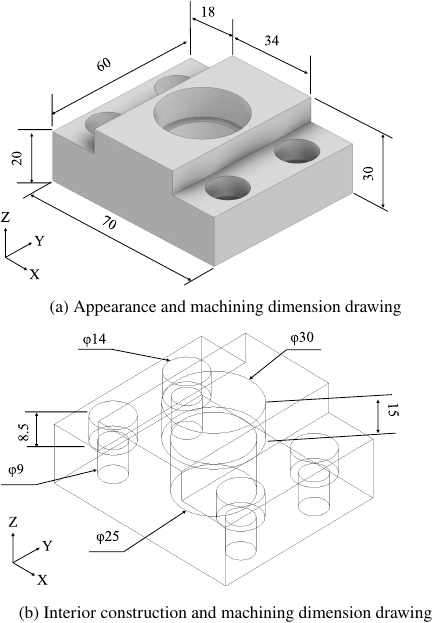
Fig. 1. Outline of machined shape of workpiece.
3. Workpiece and Process Design
We considered the manufacture of the workpiece shown in Fig. 1(a), using a drill-to-drill holes and an end mill to shoulder mill and bore a 70 \(\times\) 60 \(\times\) 30 mm piece of carbon steel (S50C). This workpiece had the shape of a holder for inserting a bearing, with an outer diameter of 30 mm, and was anchored by four M8 bolts. All the machining was completed by working on the upper surface. The workpiece interior was composed of a 25 mm-diameter tiered structure to hold the bearing and 14 mm-diameter tiered structures to tighten the bolts.
The machining in this work could be executed using a minimal tool configuration consisting of an 8 mm-diameter four-flute solid end mill and a 9 mm-diameter two-flute solid drill. However, the machining time could be reduced by using tools with larger diameters. Thus, we employed a 12 mm-diameter four-flute solid-end mill, 16 mm two-flute end mill, and 20 mm two-flute drill, as shown in Fig. 2, to consider multiple tool configurations. Our previous study 27 found that throwaway tools are preferable to solid tools in terms of the tool cost and environmental load. Therefore, we employed throwaway tools for the 16 mm-diameter end mill and 20 mm-diameter drill, which are readily available in the market. The base materials of the tools and indexable inserts were cemented carbides. The 9 mm-diameter drill had an (Al,Ti,Cr)-based multilayer coating, whereas the other tools had (Al,Ti)-based coatings. The coatings of all the tools were intended for use on steel materials.
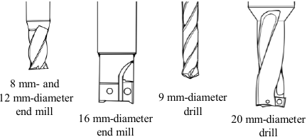
Fig. 2. Shapes of tools used in experiment.
The process design for the various tool configurations was performed by setting the machining features and tool paths using CAM. To minimize the additional setup time due to tool changes, machining steps that could be executed by the same tool were carried out contiguously. To machine circles, a drill was first used to drill a pilot hole, which was then expanded using an end mill with a smaller diameter than the hole. The cutting velocities, \(v_c\) [m/min], and feed rates, \(f\) [mm/rev], recommended by the tool manufacturer were adopted as the cutting conditions. Based on these rules, we planned four machining processes, as illustrated in Figs. 3 and 4. Case 1 was based on the configuration with the minimal number of tools, which consisted of an 8 mm-diameter end mill and a 9 mm-diameter drill, and was positioned as the reference case. Case 2 additionally employed a 12 mm-diameter end mill to remove the upper material with a higher efficiency compared to that in Case 1, thus shortening the machining time. The other machining steps were executed as in Case 1 using the 8 mm-diameter end mill and 9 mm-diameter drill. Case 3 included a 20 mm-diameter drill, which made it possible to use a 12 mm-diameter end mill to machine the central hole and further reduce the machining time. Case 4 also employed a 16 mm throwaway end mill to improve the removal rate using a large-diameter tool.
When using the 8 mm- and 12 mm-diameter solid end mills, we set two machining patterns: Mode A and Mode B. With \(D_c\) denoting the tool diameter, Mode A consisted of shoulder milling with radial depth of cut \(a_e = 0.5 D_c\) and axial depth of cut \(a_p = 0.9 D_c\). For Mode B, these were set to \(a_e = 1.1 D_c\) and \(a_p = 0.2 D_c\), respectively. The actual cutting conditions may have been less than the set cut depths because of the constraints imposed by the machined part.
The total energy consumption of each pattern was predicted using the specific energy-consumption model, and the effect of the process design on the energy consumption was quantitatively evaluated.
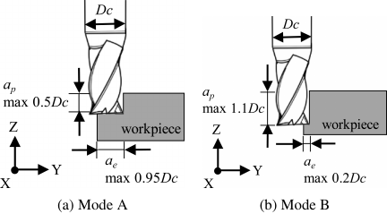
Fig. 3. Selectable modes for shoulder milling.
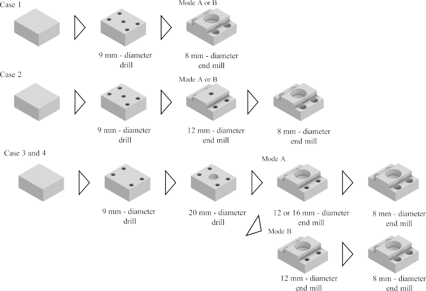
Fig. 4. Outline of machining sequences for workpiece using various process designs and conditions for Modes A and B applied to solid end mills.
4. Energy Evaluation
Figure 5 shows the transition in the power consumption from machine start-up to the completion of machining. The power consumption of the machining center was predominantly governed by the energy required for the cutting load during machining.
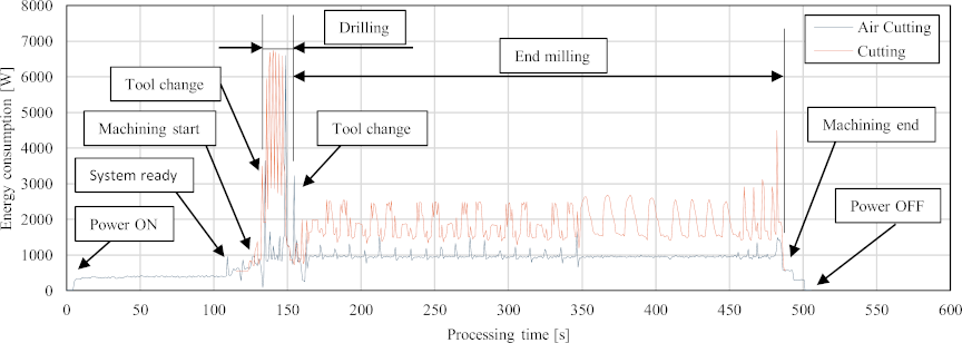
Fig. 5. Energy consumption trends during machining in Case 1, Mode A.
The total energy, \(E_\mathit{all}\) [J], consumed during the entire machining process using the three-axis vertical machining center consisted of the energy consumed during material removal, \(E_{\mathit{cut}}\) [J], energy consumed for non-machining operations, \(E_\mathit{idle}\), and energy consumed while standing, \(E_\mathit{standby}\) [J], which are expressed as follows:
Because the cutting conditions in this study involved multiple tools and modes, this can be expressed as follows:
This equation was used to perform the computations. The machining center employed in the experiment was driven by compressed air supplied by an external compressor, which was not included in the above energy calculation. Here, \(i\) \((i=1, 2, \dots, N)\) represents the tool, and \(\mathcal{I}_A\) and \(\mathcal{I}_B\) represent the sets of tools used for machining in Modes A and B, respectively.
\(E_{\mathit{cut}, i}\) can be calculated using \(P_{{\mathit{cut}},i}\) [W], the energy consumed per unit time during machining with tool \(i\), and \(t_{\mathit{cut},i}\) [s], the machining time for process \(i\), as follows:
We estimated \(P_{\mathit{cut}, i}\) using Eq. \(\eqref{eq:energy}\), and \(v_m\) could be derived by dividing the removed volume, \(V\), computed from the data used in the computer-aided design (CAD) model by the machining time, \(t_{\mathit{cut}}\), derived from the cutting simulation using the CAM program.
Table 1. Division of machining processes and task list for Case 1 using the workpiece.

\(E_\mathit{idle}\) [J] is defined as the energy consumed when the NC program runs during the time interval in which no material removal occurs. This can be expanded as follows:
Table 2. Tools used and cutting conditions applied to construct specific energy-consumption models.

\(E_\mathit{standby}\) [J] was the energy consumed to maintain the machine, including machining setup tasks such as mounting the tool, setting the tool length, setting the work coordinate system, and removing the work, along with that consumed in the standby state when the machine was not operating but the power was switched on. The main factors were the energy required to keep the CNC device running, maintain the spindle and table, and cool the device. Although the energy consumed per unit time depended on the machine configuration and control method, it remained constant, without large fluctuations. To estimate \(E_\mathit{standby}\), we used 550 W, based on measurements, as the energy consumed per unit time, and set 180 s as the tool mount time for a single tool, 120 s as the time needed to set the tool length, 180 s as that needed to set the work coordinate system, and 90 s as the time needed to mount and remove the work.
As an example of the workpiece machining process, we present the detailed tasks for Case 1 in Table 1. In this task table, the entire machining process is categorized into two processes—setup and machining—along with their accompanying tasks. The setup consists of preparatory tasks such as the loading and unloading of the material, setting the work coordinate system, and setting up the tool. Setting the work coordinate system was included in the setup process of the first task. The tool setup was performed not only in the setup process for the first task but also whenever a tool change was necessary. We assumed a tool life of 1800 s of machining time for all the tools and changed the tool in advance when it was expected to reach its life during machining.
The machining process included cutting tasks using a drill or end mill, tool changes between cutting tasks, approach tasks, and the return to the origin. The time required for each process was calculated using the CAM simulation results. Thus, drilling with the 9 mm-diameter drill involved a machining time of 7 s and approach time of 4 s, shoulder milling with an 8 mm-diameter end mill involved a machining time of 73 s and approach time of 108 s, circle milling with a 30 mm-diameter end mill involved a machining time of 28 s and approach time of 32 s, circle milling with a 25 mm-diameter end mill involved a machining time of 23 s and approach time of 24 s, and circle milling with a 14 mm-diameter end mill involved a machining time of 6 s and approach time of 16 s. The approach time was longer than the machining time in many processes because, in addition to the tool withdrawal and reapproach, the finish machining time, during which material removal rate \(v_m\) was extremely low, was defined as part of the approach maneuver. We did this because we found that this approach consumed 1500 W, whereas finish machining consumed 1550 W.
5. Construction of Power-Consumption Model
5.1. Preliminary Experiment
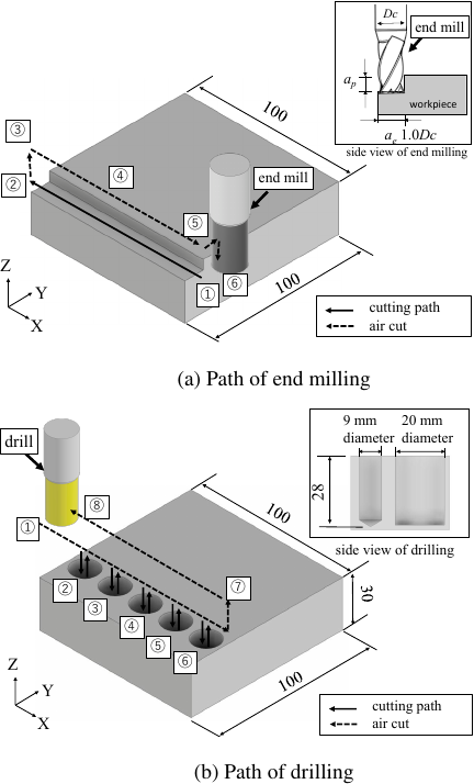
Fig. 6. Tool machining path diagrams used to construct prediction model.
We conducted a cutting experiment using carbon steel (S50C) to construct a model for predicting the energy consumed during machining using a machining center. We constructed models for each of the tools shown in Fig. 2 to evaluate the energy consumption with high accuracy. To carry out the experiment, we measured the energy consumption when machining was carried out under the cutting conditions presented in Table 2. Five levels were set for the cutting velocities and tool feeds by adopting the recommended figures in the tool catalogue of the manufacturer as the maximum (100%) values, and then reducing these in 7.5% steps down to 70% of the maximum values. Thus, each tool was used under 25 conditions in the cutting experiment. All the cutting operations were performed under wet conditions, i.e., with the use of a cutting fluid. The coolant was externally supplied to the solid end mills. It was supplied to the throwaway end mill and drill using the through-spindle method.
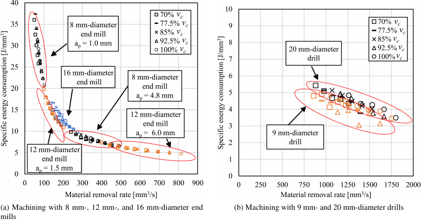
Fig. 7. Measurement results for material removal rate \(v_m\) and specific energy consumption \(c\) for various tools.
Table 3. Specific energy consumption \(c\) and power-law models for each tool.

The cutting paths of the tools are shown in Fig. 6. End milling, as shown in Fig. 6(a), consisted of shoulder milling, in which the radial depth of cut was set equal to the tool diameter, \(D_c\). The axial depth of the cut was set at 0.125\(D_c\). Because the solid end mills were capable of greater axial depths of cut, settings of 0.6\(D_c\) and 0.5\(D_c\) were also used for the 8 and 12 mm-diameter end mills, respectively. The drill shown in Fig. 6(b) was used to drill 28 mm-deep blind holes via a single feed.
The energy consumption was measured at the main circuit breaker (three-phase three-wire system) of the machining center. The measurement system included voltage/current input modules (NI9225 and NI9201), a platform (NI cDAQ-9174) manufactured by NI, and a measurement program written in LabVIEW. The voltage was measured by directly connecting the input module and power source via an O-ring terminal and lead wires. The current was measured using a clamp-on sensor. The platform synchronized the data measured by the input modules and transmitted them to a PC. The sampling rate was set at 60 Hz.
5.2. Energy-Consumption Measurement Results
The amounts of energy consumed under various cutting conditions are shown in Fig. 7, where the values are plotted on the \(v_m\)–\(c\) plane. For end milling, \(v_m\) was in the range of 48–830 mm\(^3\)/s. The energy consumed during end milling, as shown in Fig. 7(a), shows that c decreased with increasing \(v_m\), indicating that the energy required for material removal decreased with the increasing cutting velocity.
Next, drilling was considered, as shown in Fig. 7(b). During drilling, \(v_m\) was in the range of 800–1800 mm\(^3\)/s, indicating that the material was removed at more than twice the efficiency of end milling. As in the case of end milling, \(c\) decreased with increasing \(v_m\) for either tool. Compared to end milling, drilling had a low \(c\) even in the high \(v_m\) range, suggesting its superiority from the standpoint of energy efficiency. This indicated that drilling should be prioritized in the process design.
5.3. Regression Model
Based on the results shown in Fig. 7, we derived a regression model in which the specific energy consumption, \(c\), was expressed by a power law. Table 3 presents the specific energy consumption models derived for each tool and their corresponding coefficients of determination, \(R^2\). We found that \(R^2 > 0.88\) for the end mills, indicating a high goodness of fit. In drilling, although \(R^2 > 0.85\) for the 20 mm-diameter tool, we found that \(R^2 = 0.61\) for the 9 mm-diameter tool, which indicated that the goodness of fit was limited. This was because each drilling task required less than 2 s. Thus, the 60 Hz sampling rate was insufficient to carry out a detailed analysis. We believe that the accuracy could be improved by improving the sampling or experimental conditions.
In addition, we constructed a power consumption model from Eq. \(\eqref{eq:c1}\) and the specific energy consumption model. The results are summarized in Table 3. The specific energy consumption models were used to predict the energy consumed during machining.
6. Evaluation Results
6.1. Energy Consumed During Machining
We computed the total energy consumption values from the prediction model for Cases 1–4, which represented the different tool configurations.
Table 4 lists the predicted machining times, \(t_{\mathit{cut}}\), and total energy consumption \(E_{\mathit{cut}}\) for each case. The material removal rate, \(v_m\), used to derive the predicted values was computed by dividing the volume removed by the \(t_{\mathit{cut}}\) value obtained from the CAM simulation.
In each case, Mode A yielded lower values for \(t_{\mathit{cut}}\) and \(E_{\mathit{cut}}\) than Mode B. This was because the value of \(v_m\) was larger than that of Mode B, resulting in greater energy efficiency. Specifically, in Case 1, the \(t_{\mathit{cut}}\) value of Mode B (676 s) was reduced to approximately half (350 s) in Mode A, whereas \(E_\mathit{cut}\) was reduced from 1231kJ to 688kJ. Similar trends were observed in Cases 2 and 3. The lowest \(t_{\mathit{cut}}\) and \(E_{\mathit{cut}}\) values were found in Case 3, Mode A, which can be regarded as the most efficient process setting. In Case 4, which employed a 16 mm-diameter end mill, it was not possible to set a large depth of cut, \(a_p\), owing to the inserted flute. Thus, \(t_{\mathit{cut}}\) was 591 s and \(E_{\mathit{cut}}\) was 1079kJ. Although a large-diameter tool was used, this did not result in energy-efficient machining owing to the characteristics of the throwaway tool. These results showed that different process designs and machining conditions significantly affect the energy consumption, and that the value of \(v_m\) directly affects the energy efficiency.
Table 4. Predicted machining time and total energy consumption values with different process designs.

Next, the predictions were compared with the actual measured power-consumption values for each case to examine the validity of the model predictions. Figs. 8 and 9 show the measured and predicted values, respectively, for each case. The abscissas of the graphs represent the machining time [s], and the ordinates represent the power consumption [W] of the entire machining center, where the measurements and model predictions are presented together. In Case 1, which used an 8 mm-diameter end mill, the power consumed per unit time during profile machining, where the greatest volume of material was removed, was kept low, and the measured power was stable at approximately 2600 W in Mode A and approximately 1800 W in Mode B. Because the power consumption model yielded the average power consumption of the removed region, no fluctuations in the power consumption arose. When the predicted and measured values were compared, the means of the peak and valley measurements for the machining task agreed well with the predictions.
In Case 2 (Modes A and B), the addition of the 12 mm-diameter end mill to the tool configuration of Case 1 improved the efficiency of the early-stage processing of the workpiece and reduced the machining time. While this also caused the appearance of regions with large power consumption exceeding 3000 W, when compared to Case 1, the total energy consumption was approximately the same or slightly lower than that of Case 1. The predicted peak values agreed with the measurements in terms of both timing and magnitude.
In Case 3 (Modes A and B), the introduction of the 20 mm-diameter drill further shortened the time required to drill the central hole, as well as the total machining time. The machining time for Mode A was 280 s, which was the shortest time for all the cases. The machining load for boring the central section with the 12 mm-diameter end mill was less than 2500 W, which was lower than that when using the 8 mm-diameter end mill. The prediction model successfully reproduced the power fluctuations caused by the addition of the tool.
Case 4 used a 16 mm-diameter throwaway end mill for grooving, and the maximum tool depth of cut, \(a_p\), was small at 0.125\(D_c\), although a large-diameter tool was used, which increased the total machining distance and extended the machining time to 630 s. However, there were no high-load regions exceeding 3000 W, with relatively mild power fluctuations. The prediction model also successfully reproduced the power fluctuations, thereby verifying a certain degree of compliance.
In summary, the prediction model agreed well with the measurements in all cases, demonstrating its validity in quantitatively capturing the changing energy consumption characteristics depending on the tool configuration. However, the CAM simulation produced machining times that did not agree with the measured data. In particular, the predicted machining times for Mode A were approximately 40 s shorter than the actual measurements. This was most likely because the characteristics of the drive shaft of the machining center were not reflected in the simulations. The tool rapid-traverse velocity of the machining center was 9000 mm/min for the \(\mathit{XY}\)-axes and 7500 mm/min for the \(Z\)-axis. However, in the simulation, it was only possible to set the same velocity for the \(\mathit{XYZ}\)-axes, which we set to 9000 mm/min. As a result, the number of rapid tool traverses increased in Mode B because of its lower \(v_m\) value. The velocity difference along the \(Z\)-axis thus lowered the predicted machining time. Additionally, a discrepancy was observed between the predicted and measured peak power values. This occurred because the data obtained from the CAM system were limited to the total cutting time and rapid feed time for each process, making real-time calculations of \(v_m\) difficult. Therefore, in this study, the power consumption was estimated based on the average \(v_m\) for each process, which resulted in the observed discrepancy.
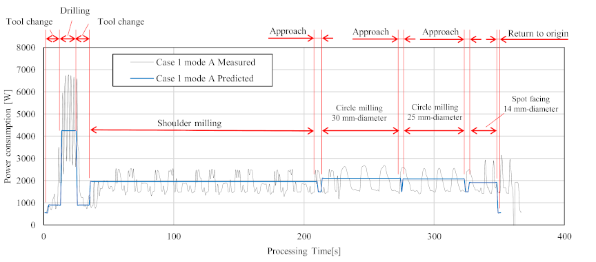
Fig. 8. Predicted and measured power consumption values for each machining process in Case 1, Mode A.
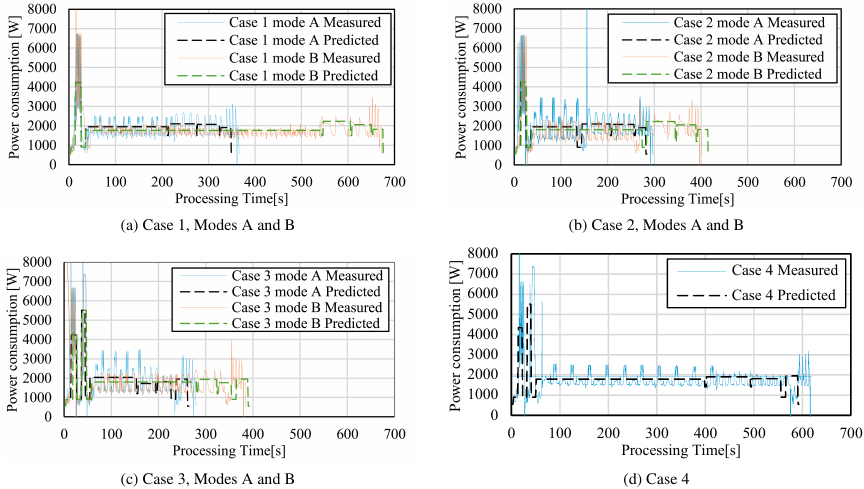
Fig. 9. Measured and predicted amounts of energy consumed to machine workpiece.
6.2. Production Volume and Energy Consumption
The share of the energy consumption (\(E_\mathit{standby}\)) that arose from the setup and miscellaneous operations, as evaluated in this study, varied depending on the number of manufactured products. Therefore, we evaluated the energy consumption, \(E_\mathit{all}\), of scenarios in which 10, 20, …, and 100 workpiece units were manufactured.
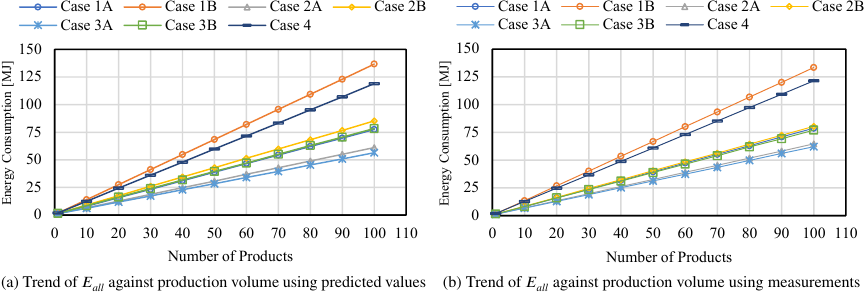
Fig. 10. Trend of total energy consumption \(E_\mathit{all}\) against number of products.
Figure 10 shows the change in energy consumption with the number of products. Fig. 10(a) shows the values computed using the energy-consumption model constructed in this study. For comparison, Fig. 10(b) presents the data obtained from the measurements. In both cases, the energy consumption increased linearly with the number of products, reflecting the fact that the machining conditions and shapes were constant. The estimated energy values obtained using the prediction model displayed the same tendencies as the measurements. In particular, the shoulder milling time for the upper part of the work involved a long path in Mode B for Cases 1 and 3, as well as in Case 4. In these cases, the maximum error from the measurements was 6%, confirming the high reliability of the prediction model.
Meanwhile, a maximum error of approximately 10% occurred in Case 3 (Mode A), which had a shorter machining time. This was because the approach maneuver had a higher share relative to the machining time in this case; therefore, the effect of the non-machining time could not be ignored. As a result, factors that could not be dealt with using a model that only considered the energy consumption during machining caused a difference between the predicted and measured values.
When the relations between the production volumes and energy consumption values during mass production were compared, we found that Case 3, Mode A, had the lowest energy consumption. In both the predicted and measured results, the final energy required for mass production was approximately 60 MJ, thus displaying a high efficiency compared to the other conditions. This was followed by Case 2, Mode A. In both cases, shoulder milling of the upper part of the workpiece was executed quickly owing to the high \(v_m\). Cases 1 (Mode B) and 4 had high energy-consumption values, consuming 100–125 MJ to manufacture 100 units. These cases had machining times exceeding 590 s, which was approximately twice that of Mode A in Cases 2 and 3. The effect of the accumulation of \(E_\mathit{all}\) caused by a longer machining time was greater than that in cases in which a high \(v_m\) temporarily caused high peak power values. When prototyping a single unit, however, the predicted value was 1.19 MJ in Case 2, Mode A, and 1.30 MJ in Case 3, Mode A. The greatest energy efficiency was achieved, at 1.17 MJ, in Case 1, Mode A, which had the minimal tool configuration. This resulted from the difference in the setup time (i.e., \(E_\mathit{standby}\)) owing to the tool configuration. However, Case 2, Mode A, was the most efficient when producing two units, and Case 3 was the most efficient when producing three or more units.
Overall, the effect of \(E_{\mathit{cut}}\), which was proportional to the machining time, was the dominant factor when estimating the energy consumption. Therefore, reducing the machining time directly improved the energy efficiency in all production stages.
Table 5. List of market prices of tools.

Table 6. Number of tools used for each workpiece production quantity.

6.3. Economic Cost and Productivity
When considering the actual manufacture of products, in addition to the energy consumed by the machine, it is necessary to consider the tool costs, labor costs, and productivity. In particular, the complexity of the setup has a significant effect on the production efficiency in a process design that involves diverse tools. Thus, the economic costs and total machining times (makespans) were evaluated in scenarios in which a single unit of the workpiece was prototyped and 10, 20, \(\ldots\), 100 units were mass-produced. We considered the labor costs of the machine operator, tool costs, and energy consumption costs to evaluate the economic costs. We assumed a labor cost of 2000 JPY per hour. We computed the number of required tools from the cutting times for each case and evaluated the tool costs based on the market prices of the tools, as listed in Table 5. The solid tools were changed along with their tool bodies, whereas the throwaway tools were changed by replacing only the insert. Thus, the cost of the tool body only had to be considered once in the case of a throwaway tool. To evaluate the productivity, the number of required tool changes was counted for each case, from which the total setup time was estimated for inclusion. The tool life was assumed to represent a realistic value based on the cutting conditions and tool life recommended by the tool manufacturer. In this study, relatively high-efficiency cutting conditions were assumed, and the tool life was set to 1800 s. The following values were used as the cutting distances until the end of the tool life: 23.97 m for the 8 mm-diameter end mill, 21.54 m for the 12 mm-diameter end mill, 16.71 m for the 16 mm-diameter end mill, 45.59 m for the 9 mm-diameter drill, and 10.31 m for the -diameter drill. Tool replacement was performed after the “Return to Origin” operation. Table 6 lists the number of tool replacements for each case. The energy cost was set to 15.73JPY/kWh, based on the industrial electricity rate of Kansai Electric Power Company in Japan (2025).
Figures 11 and 12 show how the economic costs varied with the production volume. The costs increased with the number of products. The main factor was the tool cost. The initial cost was the highest for Case 4, owing to the use of throwaway tools for the 16 mm-diameter end mill and 20 mm-diameter drill. The tool bodies of these tools are more expensive than those of solid tools, thereby increasing the initial cost. However, because only the insert needed to be changed, Case 4 became the most cost-effective case for production volumes greater than approximately 50 units. The total cost increased the most with greater volumes in Case 1, Mode B, which used a minimal tool configuration consisting of a 9 mm-diameter drill and an 8 mm-diameter end mill. Because the 8 mm-diameter end mill had to cover a lengthy machining distance, it reached its service life relatively quickly and had to be changed frequently, which was the main factor for the cost increase. Case 2, Mode B, and Case 3, Mode B, were also relatively costly. Both cases employed Mode B with a low \(v_m\), which lengthened the machining time compared to Mode A in the respective cases. Consequently, the number of tool changes increased because of the tool life, and the total cost exceeded 380,000 JPY. In all cases, the proportion of the “energy consumption cost” was very small, and even when 100 workpieces were produced, the maximum cost was as low as approximately 600 JPY. These findings indicated that reducing the number of tool setup processes is important for small-lot production machining methods, with a high \(v_m\) being highly effective in reducing costs.
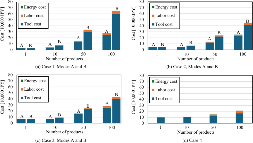
Fig. 11. Breakdown of economic costs for each workpiece production quantity.
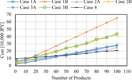
Fig. 12. Trend of economic cost against number of workpieces produced.
Figure 13 shows how the makespan varied with the production volume. The graphs show a linear tendency, where the machining time increased proportionally with the number of products. This stemmed from the fact that the machining time per unit remained virtually constant because the machining conditions were constant for all the products, and the workpiece shape was the same. This suggested that when planning the machining time or evaluating the production capacity under mass-production conditions, it is appropriate to make estimates based on the effective cutting time, which allows for accurate scheduling at the process-design stage. However, it is also necessary to account for non-machining time, such as for setup and tool changes, in small-lot production or prototyping. Thus, Case 1, which employed two tools, required 600 s for setup, including tool mounting, whereas Cases 3 and 4, each of which employed four tools, required 1200 s for setup, or approximately twice the time. Therefore, when the setup time is considered, Mode A had the shortest machining time when producing a single unit. In other words, the effect of the non-cutting time, such as that required for setup, becomes diluted on a per-unit basis and is relatively negligible in the case of mass production. Thus, an evaluation based mainly on the cutting time becomes valid, whereas improving the setup efficiency is directly connected to increased productivity in the case of small-lot production.
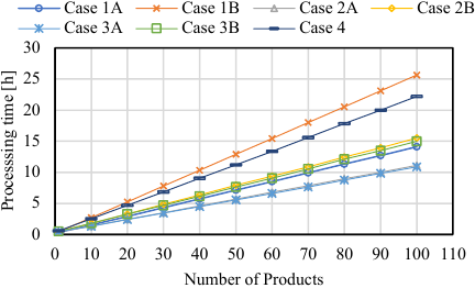
Fig. 13. Trend of total machining time against number of workpieces produced.
Finally, we discuss the makespan and economic costs from the perspective of energy efficiency. The total energy consumption for mass production could be estimated as the accumulation of \(E_\mathit{all}\), which greatly depended on the machining time. Therefore, the makespan and total energy consumption displayed similar trends. Case 2, Mode A, and Case 3, Mode A, both displayed superior performances for these parameters. In terms of the economic cost, reducing the machining time reduced the number of tool changes needed because of reaching the end of the tool life. Thus, as in the case of the makespan, Case 2, Mode A, and Case 3, Mode A, were relatively advantageous from a cost standpoint. However, although Case 4 involved a long machining time and frequent tool changes, it achieved the lowest economic cost in mass production because it was only necessary to change the low-cost insert. As this shows, the optimal conditions for energy efficiency and economic costs are not necessarily the same, and we see that tool configuration and tool changes owing to the service life have significant effects on the cost evaluation. Furthermore, in the case of small-lot production, such as single-unit production, simplifying the tool configuration, as in Case 1, Mode A, results in a short setup time and may achieve high-efficiency processing in terms of the energy efficiency, makespan, and economic costs.
7. Conclusion
In this study, we focused on process design to improve the energy efficiency of a machining process using a three-axis machining center. We used a specific energy consumption model to evaluate the total energy consumed during the manufacture of a workpiece using multiple tool configuration patterns. We found that the energy consumed by non-machining processes, such as setup and tool preparation, accounted for a sizable, non-negligible portion in the case of small-lot production. In such cases, reducing the number of tools and shortening the setup time were effective in reducing the energy consumption. Meanwhile, the effect of the time required for the setup and tool changes was diluted in the case of mass production, where the energy consumed during machining was the main energy consumption factor, and the total energy consumption was virtually proportional to the machining time. Therefore, the selection of a tool configuration that shortens the machining time is preferable from the standpoint of energy efficiency, although the setup time may increase. As shown, we found that it is possible to carry out an energy-saving process design using a specific energy consumption model. This finding constitutes a concrete measure that can be implemented at the machining-process level to create a carbon-neutral society.
Another issue that must be addressed in the future is improving the prediction accuracy for non-machining energy, such as that involved in the approach maneuver. In this study, we adopted representative times and energy values for the evaluation. However, these maneuvers vary depending on the machining path or tool position; thus, the estimation will include a certain amount of error. Although this may not present major problems for linear machining paths, the CAM-estimated and actual machining times may differ for curved or helical paths. It is difficult to accurately predict the machining time for such complex cutting paths, which can reduce the accuracy of the predicted material removal rate and total energy consumption. Therefore, it is necessary to develop a method to accurately acquire the traversed distance and time.
Acknowledgments
The authors wish to express their deep gratitude to Michitake Hoki at Setsunan University for his assistance in conducting the experiments.
- [1] T. Ogawa, “Building of efficient, energy-saving lines with an extremely-compact machining center and CNC lathe,” Int. J. Automation Technol., Vol.4, No.2, pp. 150-154, 2010. https://doi.org/10.20965/ijat.2010.p0150
- [2] N. Uchiyama, Y. Ogawa, and S. Sano, “Energy saving for gantry-type feed drives by synchronous and contouring control,” Int. J. Automation Technol., Vol.6, No.3, pp. 363-368, 2012. https://doi.org/10.20965/ijat.2012.p0363
- [3] K. Mori et al., “Energy efficiency improvement of machine tool spindle cooling system with on-off control,” CIRP J. of Manufacturing Science and Technology, Vol.25, pp. 14-21, 2019. https://doi.org/10.1016/j.cirpj.2019.04.003
- [4] B. Denkena et al., “Energy efficient supply of cutting fluids in machining by utilizing flow rate control,” CIRP Annals, Vol.72, Issue 1, pp. 349-352, 2023. https://doi.org/10.1016/j.cirp.2023.04.082
- [5] M. Fujishima, H. Shimanoe, and M. Mori, “Reducing the energy consumption of machine tools,” Int. J. Automation Technol., Vol.11, No.4, pp. 601-607, 2017. https://doi.org/10.20965/ijat.2017.p0601
- [6] A. M. M. Ullah et al., “Strategies for developing milling tools from the viewpoint of sustainable manufacturing,” Int. J. Automation Technol., Vol.10, No.5, pp. 727-36, 2016. https://doi.org/10.20965/ijat.2016.p0727
- [7] A. Hayashi, F. Arai, and Y. Morimoto, “Simulation of energy consumption during machine tool operations based on NC data,” Int. J. Automation Technol., Vol.15, No.6, pp. 764-773, 2021. https://doi.org/10.20965/ijat.2021.p0764
- [8] K. Fang et al., “A new approach to scheduling in manufacturing for power consumption and carbon footprint reduction,” J. of Manufacturing Systems, Vol.30, No.4, pp. 234-240, 2011. https://doi.org/10.1016/j.jmsy.2011.08.004
- [9] T. Samukawa and H. Suwa, “An optimization of energy-efficiency in machining manufacturing systems based on a framework of multi-mode RCPSP,” Int. J. Automation Technol., Vol.10, No.6, pp. 985-992, 2016. https://doi.org/10.20965/ijat.2016.p0985
- [10] M. Ertem, “Renewable energy-aware machine scheduling under intermittent energy supply,” IEEE Access, Vol.12, pp. 23613-23625, 2024. https://doi.org/10.1109/ACCESS.2024.3365074
- [11] M. K. Chinnathai and B. Alkan, “A digital life-cycle management framework for sustainable smart manufacturing in energy intensive industries,” J. of Cleaner Production, Vol.419, Article No.138259, 2023. https://doi.org/10.1016/j.jclepro.2023.138259
- [12] B. Denkena et al., “Energy efficient machine tools,” CIRP Annals, Vol.69, Issue 2, pp. 646-667, 2020. https://doi.org/10.1016/j.cirp.2020.05.008
- [13] T. Samukawa and H. Suwa, “Energy efficiency assessment using material removal rate and its application to wet and dry end-milling.” J. of the Japan Society for Precision Engineering, Vol.91, No.5, pp. 579-585, 2025. https://doi.org/10.2493/jjspe.91.579
- [14] T. Matsumura et al., “Predictive cutting force model and cutting force chart for milling with cutter axis inclination,” Int. J. Automation Technol., Vol.7, No.1, pp. 30-38, 2013. 10.20965/ijat.2013.p0030
- [15] H. Narita, “A method for using a virtual machining simulation to consider both equivalent CO2 emissions and machining costs in determining cutting conditions,” Int. J. Automation Technol., Vol.9, No.2, pp. 115-121, 2015. https://doi.org/10.20965/ijat.2015.p0115
- [16] L. Hu et al., “Minimising the machining energy consumption of a machine tool by sequencing the features of a part,” Energy, Vol.121, pp. 292-305, 2017. https://doi.org/10.1016/j.energy.2017.01.039
- [17] Y. Oda, M. Fujishima, and Y. Takeuchi, “Energy-saving machining of multi-functional machine tools,” Int. J. Automation Technol., Vol.9, No.2, pp. 135-142, 2015. https://doi.org/10.20965/ijat.2015.p0135
- [18] A. Fysikopoulos et al., “On a generalized approach to manufacturing energy efficiency,” Int. J. of Advanced Manufacturing Technology, Vol.73, pp. 1437-1452, 2014. https://doi.org/10.1007/s00170-014-5818-3
- [19] T. Gutowski, J. Dahmu,s and A. Thiriez, “Electrical energy requirements for manufacturing processes,” Proc. of 13th CIRP Int. Conf. on Life Cycle Engineering, 2006.
- [20] S. Kara and W. Li, “Unit process energy consumption models for material removal processes,” CIRP Annals, Vol.60, pp. 37-40, 2011. https://doi.org/10.1016/j.cirp.2011.03.018
- [21] Y. Guo et al., “Optimization of energy consumption and surface quality in finish turning,” Procedia CIRP, Vol.1, pp. 512-517, 2012. https://doi.org/10.1016/j.procir.2012.04.091
- [22] L. Li, J. Yan, and Z. Xing, “Energy requirements evaluation of milling machines based on thermal equilibrium and empirical modelling,” J. of Cleaner Production, Vol.52, pp. 113-121, 2013. https://doi.org/10.1016/j.jclepro.2013.02.039
- [23] S. Velchev et al., “Empirical models for specific energy consumption and optimization of cutting parameters for minimizing energy consumption during turning,” J. of Cleaner Production, Vol.80, pp. 139-149, 2014. https://doi.org/10.1016/j.jclepro.2014.05.099
- [24] M. P. Sealy et al., “Energy consumption and modeling in precision hard milling,” J. of Cleaner Production, Vol.135, pp. 1591-1601, 2016. https://doi.org/10.1016/j.jclepro.2015.10.094
- [25] T. Samukawa and H. Suwa, “A basic study of predicting in-process energy consumption in machining based on specific energy consumption,” J. of the Japan Society for Precision Engineering, Vol.83 No.4, pp. 367-374, 2017 (in Japanese). https://doi.org/10.2493/jjspe.83.367
- [26] T. Samukawa, K. Shimomoto, and H. Suwa, “Estimation of in-process power consumption in face milling by specific energy consumption models,” Int. J. Automation Technol., Vol.14 No.6, pp. 951-958, 2020. https://doi.org/10.20965/ijat.2020.p0951
- [27] K. Shimomoto, Y. Otomura, and T. Samukawa, “Effect of drilling conditions on CO2 emissions,” J. of the Japanese Society for Experimental Mechanics, Vol.23, No.1, pp. 45-50, 2023 (in Japanese). https://doi.org/10.11395/jjsem.23.45
This article is published under a Creative Commons Attribution-NoDerivatives 4.0 Internationa License.